Update – I have broken this article into 2 parts (separating continuum specific normalization) for digestibility 🙂 – you can find the part II here

Normalization is critical for anything data, data analysis, data science, ML and definitely NN but normalization techniques vary for data, data type and model / process downstream where we want to leverage that data.

The aim of this article is to cover the concept of normalization, walk through different techniques, what they do and where to use them as well as proceed to some data specific normalization techniques hoping to give you some insights on how to work with them, so, lets start with the basics, what is normalization?

Normalization is the process of transforming data to a ‘standard scale’ keeping the relative information intact (i.e. without distorting the difference in values and keeping critical information intact).

This could mean scaling values between 0 and 1, centering them around 0, or adjusting them relative to some baseline (you decide the standard scale). In the context of spectra, it often means removing the baseline ‘continuum’ so the sharp features (like absorption/emission lines) stand out clearly.

Now, why is this important? Having a standard scale is important for visually interpreting and comparing things, some metrics and methods assume certain distributions and scales and if we’re training a model, standardizing data introduces numerical stability in the models, helps gradient convergence and could even help better identify features and outliers. The right normalization technique can significantly improve signal clarity and model performance.

Which one to chose? There is no one answer, the decision usually depends on

• The type of data (images, time series, spectra (scientific data), categorical, etc.)

• The goal (visual clarity, comparability, feature extraction, feeding into ML models)

• The model or algorithm downstream (linear regression cares about scale, tree models don’t)

If you prefer a brief overview, here is a summary I created with the help of notebookLM :

Dataset

In this example, we’re working with resampled spectral data from the Sloan Digital Sky Survey (SDSS), mapped to a common wavelength grid from 3800 to 9200 Angstroms across 3600 bins. This preprocessing ensures consistent input size and resolution for comparative and statistical analysis.

Spectra is rich, continuous, structured data, it capture physical information about stars (like temperature, composition, and velocity) by measuring how light intensity varies with wavelength. Its messy! different days, different instruments, different atmosphere, different stars, interstellar objects can create all sorts of variations and noise.

Why this data? Simple, because I was already working with it, and its a good use case because, its continuous and messy and requires a lot of pre processing, it has a physical meaning and is sensitive to accuracy – we need to align specific spectral lines to fingerprint a star! You can read more about the topic here or in my upcoming article on the project (some initial code for the whole project here).

Our spectral data could look like this:

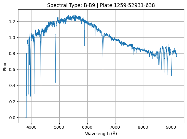
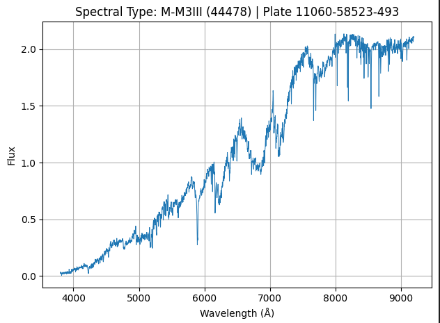
Where each of the above image represents the spectrum of a star (1 sample of our data).

Overall, our sample data consists of about ~3200 stars and is distributed as:

Now lets proceed to the different normalization techniques!

For the sake of making a reference sheet and understanding what techniques are used in general, we’ll go through all of them here:

Classical Normalization Techniques

Each method has a unique philosophy, some preserve absolute features, others emphasize shape, while a few are robust to noise or outliers. The intention is to review one of the popular and well known normalization techniques in ML and see what it really does to our data.

Most of these are available by default in popular ML libraries like scikit-learn or tensorflow, here I just write the method, because its easy enough and will help you understand what’s happening better.

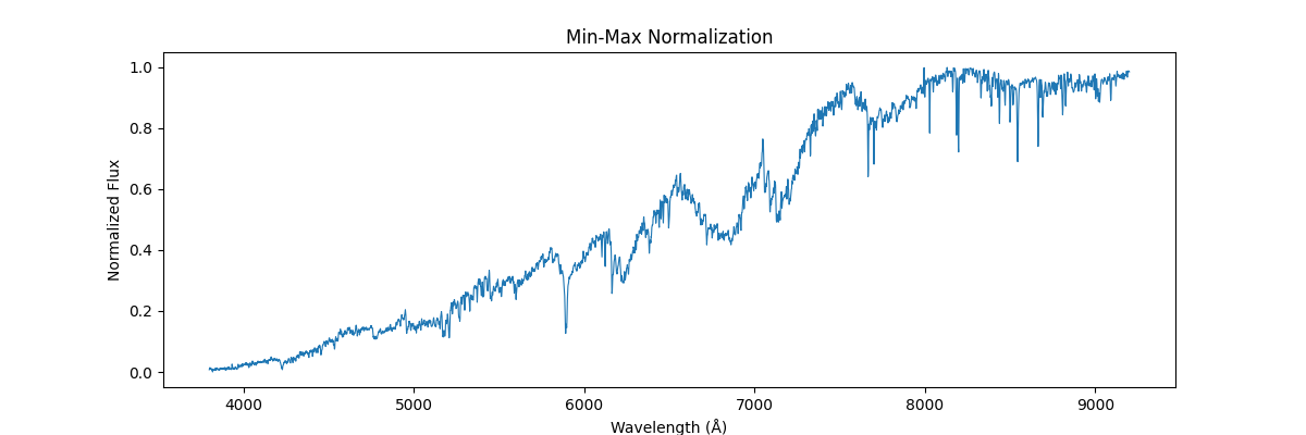
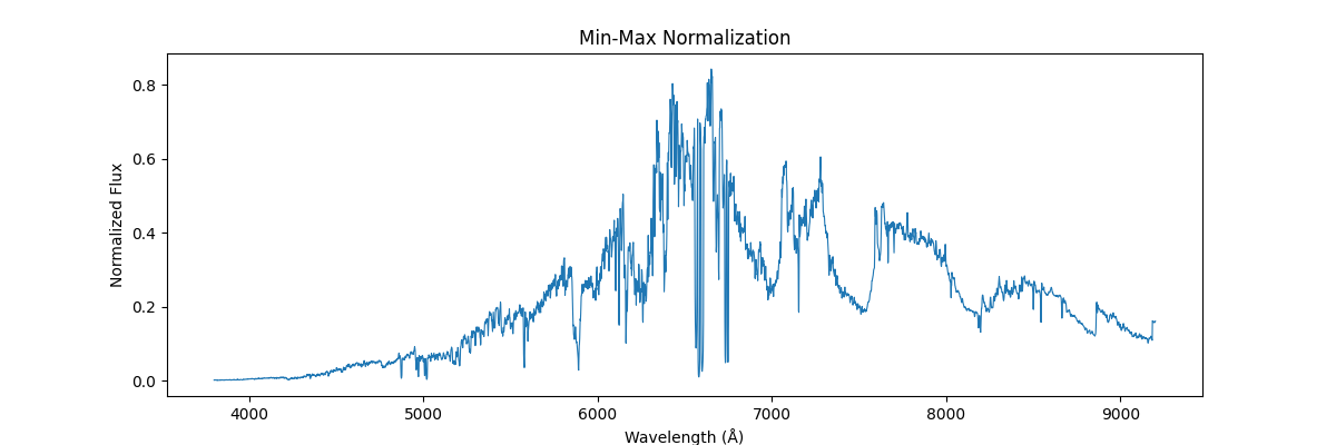
Min-Max Scaling

Method: Linearly rescales values using minimum and maximum values to the [0, 1] range. good for preserving shape and definite range of 0 and 1

(flux - min(flux)) / (max(flux) - min(flux) + 1e-8)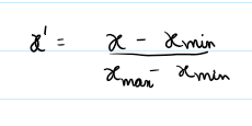

• Pros: Simple and preserves relative differences.
• Cons: Very sensitive to outliers, may suppress true variability.

def normalize_min_max(spectra):
    spectra_min = spectra.min(axis=1, keepdims=True)
    spectra_max = spectra.max(axis=1, keepdims=True)
    return (spectra - spectra_min) / (spectra_max - spectra_min + 1e-8)

Applying this on a single spectra (locally), each spectra is treated as isolated data – and the internal values are used to get the min and max – this would preserve the shape (like relative line depths and structure within the spectra) but would remove all the information which could be used to compare different spectras (like absolute flux, brightness etc.)

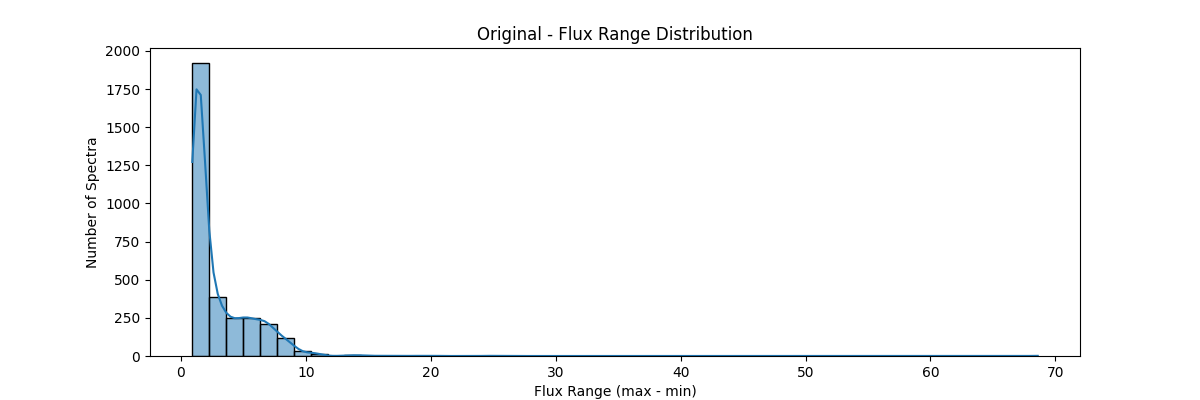
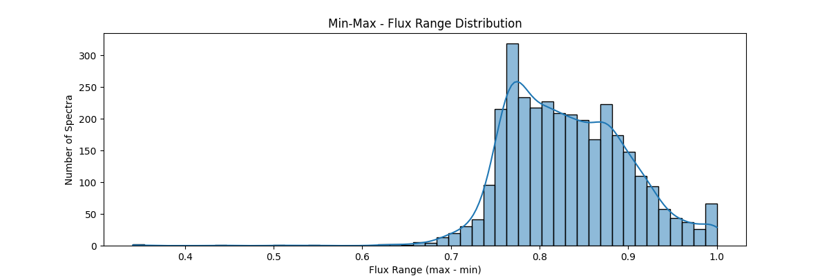
Applying this globally, that is scaling our sample relative to other samples (we use global min and max across spectras) – this would not preserve their shape but would reflect their absolute relation, how flux and brightness etc. compares to other stars

One could be fancier and apply min max class wise (its not that fancy – quite common actually for certain use cases)

If we apply our min max normalization globally – our data distribution would look something like:

Z-Score (Standard) Normalization

Method: Centers data at zero mean, unit variance. good for normal distributions

(flux - mean(flux)) / (std(flux) + 1e-8)

• Pros: Ideal for Gaussian features, useful for statistical ML.
• Cons: Still somewhat sensitive to outliers, assumes normal distribution.

def normalize_z_score(spectra):
    mean = spectra.mean(axis=1, keepdims=True)
    std = spectra.std(axis=1, keepdims=True)
    return (spectra - mean) / (std + 1e-8)

Again, applying locally,

And applying globally,

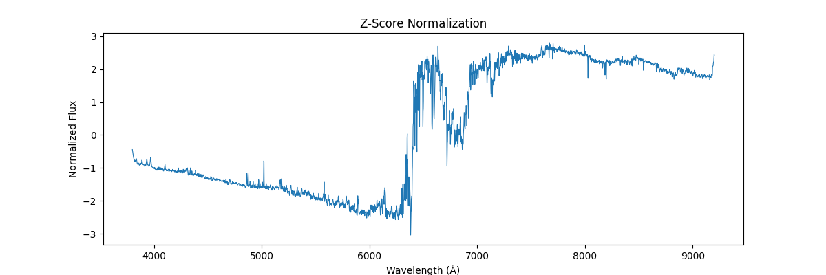
Overall distribution of data after standardization,

Area Under Curve (AUC) Normalization

Method: Normalizes based on total energy (integrated flux).

flux / (∫ flux dλ + 1e-8)

• Pros: Preserves energy distribution; useful in signal comparison.
• Cons: Can be skewed by wide continuum slopes or noise.

def normalize_auc(spectra):
    area = np.trapz(spectra, COMMON_WAVE, axis=1).reshape(-1, 1)
    return spectra / (area + 1e-8)

Applying this locally (left) and globally (right)

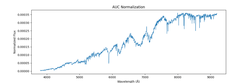
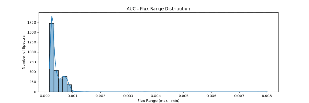
the data distribution looks somewhat like,

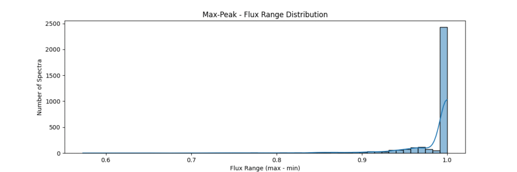
Max-Peak Normalization

Method: Divides spectrum by its maximum peak value. good for relative intensities and cases where max / peak of data are important.

flux / (max(flux) + 1e-8)

• Pros: Highlights peak intensity; good for emission line analysis.
• Cons: Dominated by a single point — poor for noise-prone data.

def normalize_max(spectrum):
    return spectrum / (np.max(spectrum) + 1e-8)

Applying this locally (left) and globally (right)

the data distribution looks somewhat like,

L2 Normalization

Method: Ensures unit vector norm in high-dimensional space. good for unit length vector use cases. (certain ML models)

flux / (||flux||_2 + 1e-8)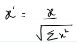

• Pros: Maintains shape in vector space, good for ML.
• Cons: Doesn’t reflect physical scale, ignores energy magnitude.

def normalize_l2(spectrum):
    norm = np.linalg.norm(spectrum)
    return spectrum / (norm + 1e-8)

Applying this locally (left) and globally (right)

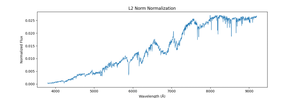
the data distribution looks somewhat like,

Robust (IQR) Normalization

Method: Uses interquartile range and median for robust scaling. handles outlier betters, median centered data (instead of mean).

(flux - median) / (IQR + 1e-8)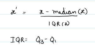

• Pros: Resists outliers and skew; ideal for noisy spectra.
• Cons: Can flatten meaningful variations outside central range.

def normalize_robust(spectrum):
    median = np.median(spectrum)
    iqr = np.percentile(spectrum, 75) - np.percentile(spectrum, 25)
    return (spectrum - median) / (iqr + 1e-8)

Applying this locally (left) and globally (right)

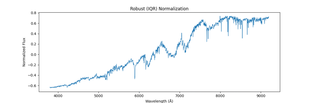
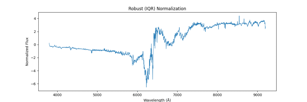
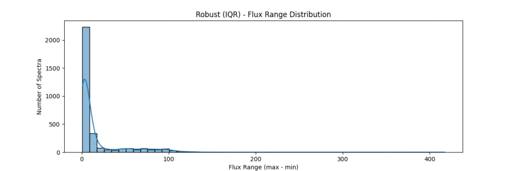
the data distribution looks somewhat like,

Log Normalization

Method: Applies log transform to compress dynamic range.

log(1 + flux)

• Pros: Dampens spikes, enhances low intensity lines.
• Cons: Loses physical interpretability, can’t handle negatives.

def normalize_log(spectra):
    return np.log1p(spectra)  # log(1 + x)

Applying this locally (left) and globally (right)

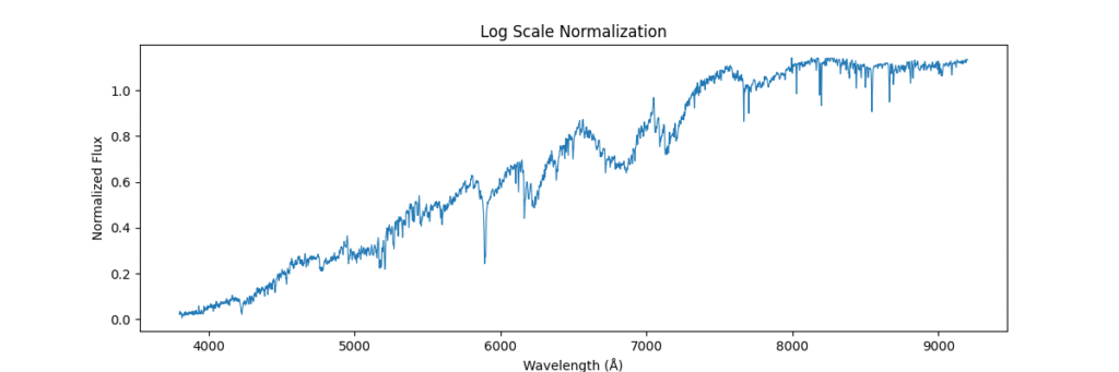
the data distribution looks somewhat like,

Quantile Normalization

Method: Aligns value ranks across spectra, forcing identical distributions. Removes technical variations between samples. Sort values, get ranks, average values at each rank across samples

• Pros: Removes inter-sample technical variation.
• Cons: Physically meaningless in spectroscopy

def normalize_quantile(spectra):
    sorted_X = np.sort(spectra, axis=1)
    ranks = np.argsort(np.argsort(spectra, axis=1), axis=1)
    avg_dist = np.mean(sorted_X, axis=0)
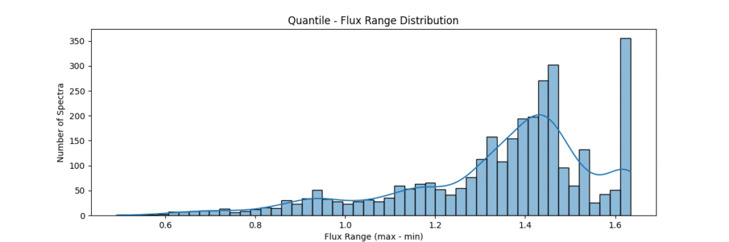
    return avg_dist[ranks]

Applying this locally (left) and globally (right)

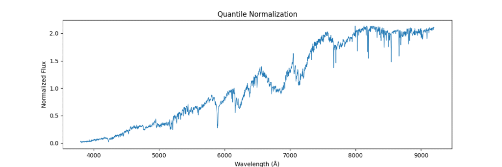
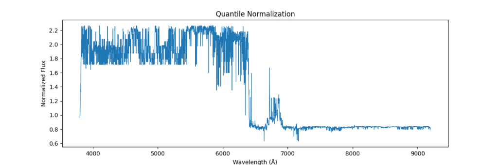
the data distribution looks somewhat like,

Conclusion

Normalization is not one size fits all. Your choice should reflect the data characteristics, application goals, and downstream models. Visual inspection is key, and automated scoring can help streamline the selection process.

You can access this code on my github repo here