I ended up writing this article after digging into a tiny rabbit hole of stellar spectra normalization (a project I picked up on a weekend and was supposed to end that weekend).
Normalization is the process of transforming data to a ‘standard scale’ keeping the relative information intact (i.e. without distorting the difference in values and keeping critical information intact).
This could mean scaling values between 0 and 1, centering them around 0, or adjusting them relative to some baseline (you decide the standard scale). In the context of spectra, it often means removing the baseline ‘continuum’ so the sharp features (like absorption/emission lines) stand out clearly.
Now, why is this important? Having a standard scale is important for visually interpreting and comparing things, some metrics and methods assume certain distributions and scales and if we’re training a model, standardizing data introduces numerical stability in the models, helps gradient convergence and could even help better identify features and outliers. The right normalization technique can significantly improve signal clarity and model performance.
This article was originally part of this Normalization post but I separated it into its own – as these details seem worth diving deeper into.
Dataset
In this example, we’re working with resampled spectral data from the Sloan Digital Sky Survey (SDSS), mapped to a common wavelength grid from 3800 to 9200 Angstroms across 3600 bins. This preprocessing ensures consistent input size and resolution for comparative and statistical analysis.
Spectra is rich, continuous, structured data, it capture physical information about stars (like temperature, composition, and velocity) by measuring how light intensity varies with wavelength. Its messy! different days, different instruments, different atmosphere, different stars, interstellar objects can create all sorts of variations and noise.
Why this data? Simple, because I was already working with it, and its a good use case because, its continuous and messy and requires a lot of pre processing, it has a physical meaning and is sensitive to accuracy – we need to align specific spectral lines to fingerprint a star! You can read more about the topic here or in my upcoming article on the project (some initial code for the whole project here).
Our spectral data could look like this:
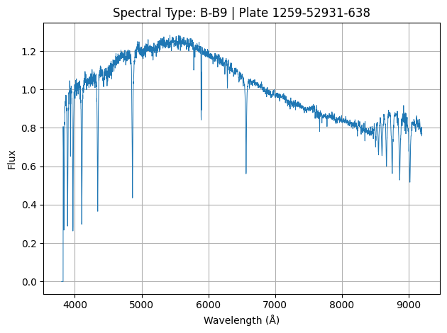
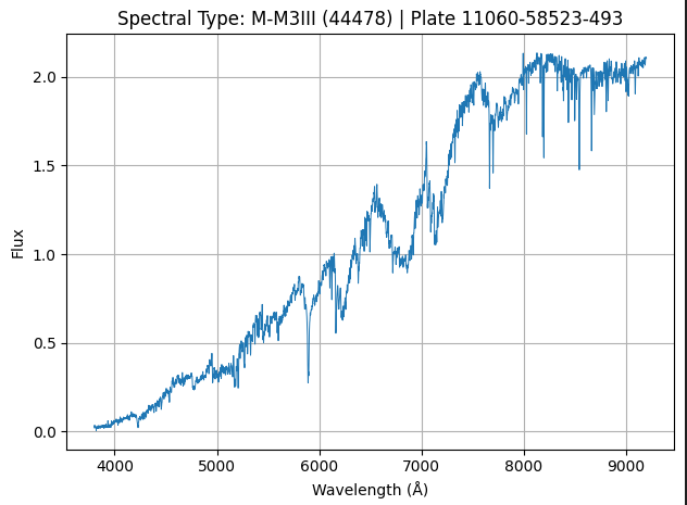
Where each of the above image represents the spectrum of a star (1 sample of our data).
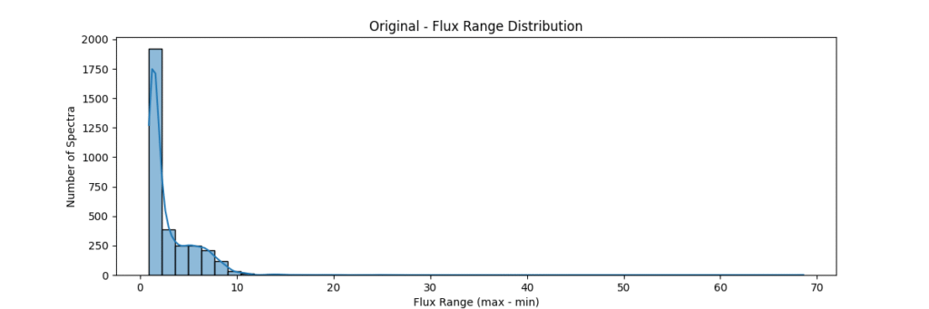
Overall, our sample data consists of about ~3200 stars and is distributed as:
Now lets proceed to the different normalization techniques!
Continuum Normalization Techniques
You can find a brief recap and summary of normalization here, lets jump into star spectrum normalization!
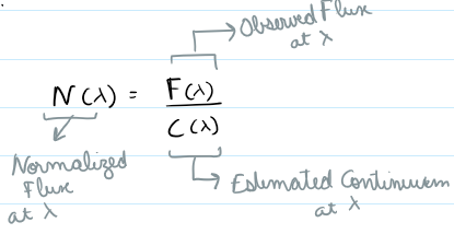
While flux normalization scales spectra globally, continuum normalization removes the baseline trend (continuum) to highlight relative features like absorption or emission lines. This is crucial in stellar classification, abundance analysis, and ML model performance on astrophysical spectra.
Savitzky Golay Filter
Method: Applies a polynomial smoothing filter (low degree polynomial over a window) to estimate the continuum, we then divide the original spectrum by this continuum to get a normalized spectra.
Library:
Scipy has an implementation which can be directly applied – as simply as:
from scipy.signal import savgol_filter
continuum = savgol_filter(flux, window_length=151, polyorder=3)
norm_flux = flux / continuum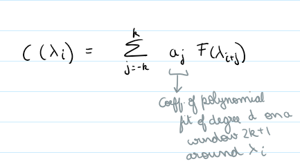
Implementation Overview:
- This function would auto select a window (10% of continuum) if not given (minimum 151 ) – window for savgol is odd
- then it identifies all the high points in the spectrum based on the given threshold ( by default we clip at 90% i.e. we keep only 10% of brightest points)
- then it creates a mask (keeping all the high points and filtering all the absorption region)
- fills the dips in the mask by interpolating
- applies smoothing filter on this data (this is savgol step – we use a windowing lower polynomial estimation for this smoothing – the order is 3 by default)
- (and ensures non zeroes) => this is our continuum
- divides the flux by the continuum to get a normalized flux
from scipy.signal import savgol_filter

def continuum_savgol(flux, window=None, poly=3, clip_percentile=90):
    # dynamically find the window based on flux -
    # and ensure its  10% of total length and atleast 151
    # (it has to be odd - to get central peak)
    if window is None: window = min(151, len(flux) // 10 | 1)
    if window % 2 == 0: window += 1

    # percentile clipping - keeping only upper X% flux values
    # (to avoid absorption dips affecting continuum)
    # only top/brightest 10% by default will disctate the continuum
    threshold = np.percentile(flux, clip_percentile)
    mask = flux > threshold

    # create a smooth baseline by interpolating over masked points
    # (since we removed absorption lines - we fill in the holes -
    # connecting the brightest points)
    interp_flux = np.copy(flux)
    interp_flux[~mask] = np.interp(np.flatnonzero(~mask), np.flatnonzero(mask), flux[mask])

    # we use savgol on our interpolated flux made of the brightest points
    # => continuum
    continuum = savgol_filter(interp_flux, window_length=window, polyorder=poly, mode='interp')
    # to avoid division by very very small numbers
    # so its not inf and ensure its not 0 or -ve
    continuum = np.clip(continuum, 1e-5, None)
    # normalized flux = flux / general curve => values between 0-1
    return flux / continuum, continuum
- Pros: Best for clean spectras with broad features, works quite fast, no need for model fitting, preserves broad shape and smooths out noise
- Cons: Can over smooth broad features (if windows too big), bad for low SNR spectra (or noisy data as noise can be part of continuum)
Spline Fit
Method: Identifies high-flux points across bins, fits a spline through them to approximate the continuum, and normalizes by the result.
spline = UnivariateSpline(wave[mask], flux[mask], s=s_factor)
continuum = spline(wave)
norm_flux = flux / continuum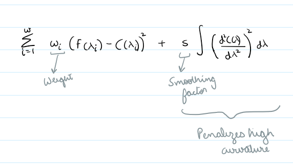
Methodology Overview:
- Initialize masks and bins (10 minimum) but its based on a bin per every 300 points
- in each bin we then select a percentile of points based on bin flux ( by default we clip at 90% i.e. we keep only 10% of brightest points)
- then we define a smoothing factor based on wave range (s=0 would mean exact interpolation through all the points and s>0 would encourage smoothing)
- then we call univariate splie fit (piecewise polynomial through the selected lines)
- its important to have a high enough s to prevent overfitting but not too high to miss important features, not have an aggressive high points percentile resulting in missing continuum in noisyregions, have decent amount of points per bin
from scipy.interpolate import UnivariateSpline

def continuum_spline(wave, flux, high_percentile=95, s_factor=1e-4):
    mask = np.zeros_like(flux, dtype=bool)

    # bin the spectrum - max 10 bins or a bin size of 300 points
    n_bins = max(10, len(flux) // 300)
    bins = np.linspace(wave.min(), wave.max(), n_bins + 1)

    # within each bin, find the high percentile flux value to identify continuum points
    # by default we only consider points above 95th percentile in each bin as continuum points
    for i in range(n_bins):
        bin_mask = (wave >= bins[i]) & (wave < bins[i+1])
        bin_flux = flux[bin_mask]
        if len(bin_flux) == 0:
            continue
        threshold = np.percentile(bin_flux, high_percentile)
        mask[bin_mask] |= (flux[bin_mask] > threshold)

    if np.sum(mask) < 10:
        raise ValueError("too few points to fit")

    # smoothing factor for spline fitting
    # dynamically adjusted based on wavelength range and number of points
    s = s_factor * (wave.max() - wave.min()) * len(wave)
    spline = UnivariateSpline(wave[mask], flux[mask], s=s)
    continuum = spline(wave)
    # to avoid division by very very small numbers so its not inf and ensure its not 0 or -ve
    continuum = np.clip(continuum, 1e-4, None)
    # normalized flux = flux / general curve => values between 0-1
    return flux / continuum, continuum
- Pros: Adapts well to variable continuum shape (much better than a basic polynomial)
- Cons: Super sensitive to masking thresholds, can fail if not enough valid points or fluctuate too much if point selection is poor
Hybrid – Spline with Savitzky Golay and Sigma Clipping
Method: Combines smoothing, sigma clipping, and bin based peak selection to choose continuum points, followed by spline fitting
# Apply median filter, then savgol, sigma clip, then spline fit on top N% points per bin
norm_flux, continuum = continuum_spline_wsavgol(wave, flux)
Methodology Overview:
- This function would auto select a window if not given (min 151 and odd)
- Then it will do a median filtering to remove local spikes
- This is followed by a savgol smoothing (low ordered windowed polynomial approximation)
- Then we do an iterative sigma clipping to remove outliers that deviate too much – we use median absolute deviation instead of standard deviation here to make it more robust to outliers (we use 2.5 sigma clipping by default)
- then we divide the data into bins
- within each bin we take the points that survived the sigma clipping (if there are no points we just take all points)
- we sort these points by flux and select the top n brightest points (10 by default)
- we standardize the wave (for stability) and select an appropriate smoothing factor and then proceed to fit a spline using our selected mask
- the above steps give us our continuum
- then we just divide our flux by the continuum baseline to get normalized flux
from scipy.interpolate import UnivariateSpline, LSQUnivariateSpline
from scipy.signal import savgol_filter, medfilt

def continuum_spline_wsavgol(wave, flux, smooth_window=None, sigma=2.5, s_factor=1e-4, top_n_per_bin=15, n_bins=20, verbose=False):
    # window selection for savgol - 10% of total length and atleast 151
    if smooth_window is None:
        smooth_window = min(151, len(flux) // 10 | 1)
    if smooth_window % 2 == 0:
        smooth_window += 1

    # initial smoothing - median filter followed by savgol
    # median filter to remove spikes (preserve edges better than savgol alone)
    init_smooth = medfilt(flux, kernel_size=15)
    # apply savgol on the median filtered data
    smoothed = savgol_filter(init_smooth, window_length=smooth_window, polyorder=3)

    # sigma clipping - remove outliers from continuum (e.g., deep absorption lines)
    # median - more robust to outliers than mean
    # 4 iterations of 2.5 sigma clipping using MAD
    mask = np.ones_like(flux, dtype=bool)
    for _ in range(4):
        residual = flux[mask] - smoothed[mask]
        mad = np.median(np.abs(residual - np.median(residual)))
        std = 1.4826 * mad if mad > 0 else 1e-5
        mask[mask] = np.abs(residual) < sigma * std
        smoothed = savgol_filter(flux * mask, window_length=smooth_window, polyorder=3)

    # bin data into 20 bins by default
    # take top 15 points by default in each bin as continuum points
    bins = np.linspace(wave.min(), wave.max(), n_bins + 1)
    cont_mask = np.zeros_like(flux, dtype=bool)
    for i in range(n_bins):
        in_bin = (wave >= bins[i]) & (wave < bins[i + 1])
        idx = np.where(in_bin & mask)[0]
        if len(idx) == 0:
            idx = np.where(in_bin)[0]
        if len(idx) > 0:
            top_idx = idx[np.argsort(flux[idx])[-min(top_n_per_bin, len(idx)):]]
            cont_mask[top_idx] = True

    # spline struggles with end points - can shoot up to infinity
    # so we force edge points (first and last 5) to avoid that
    cont_mask[:5] = True
    cont_mask[-5:] = True

    # scaled to make calculations numerically stable
    wave_scaled = (wave - wave.mean()) / wave.std()
    s = s_factor * len(wave) * np.median(flux)**2

    # mask deep absorptions
    mask = flux > np.percentile(flux, 85)

    # num_knots = 10
    # knots = np.quantile(wave[mask], np.linspace(0, 1, num_knots))
    # spline = LSQUnivariateSpline(wave, flux, knots[1:-1], k=3)

    spline = UnivariateSpline(wave_scaled[cont_mask], flux[cont_mask], s=s)
    continuum = spline(wave_scaled)
    continuum = np.clip(continuum, 1e-4, None)

    # normalize and clip
    norm = flux / continuum
    norm = np.clip(norm, 0.2, 3.0)

    if verbose:
        print(f"[spline_wsavgol] Points used: {np.sum(cont_mask)}, s={s:.2e}")

    return norm, continuum
- Pros: Robust (iterative sigma clipping and MAD handles outliers quite well)
- Cons: Computationally heavyy – requires careful selection of bins and smoothing.
Polynomial Fit
Method: Fits a low degree polynomial to the top percentile of flux values
coeffs = np.polyfit(wave_scaled[mask], flux[mask], deg)
continuum = np.polyval(coeffs, wave_scaled)
norm_flux = flux / continuum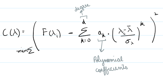
Methodology Overview:
- relatively simple – we take the highest points by flux (default 90 percentile clipping – i.e. we keep only 10% of brightest points)
- fit a polynomial through those points to get the continuum
- we divide flux by the continuum to get a normalized flux
def continuum_polynomial(wave, flux, deg=4, n_bins=25, top_n=10, clip_percentile=90):
    # scaling for numerical stability
    wave_scaled = (wave - wave.mean()) / wave.std()

    # threshold = np.percentile(flux, clip_percentile)
    # mask = flux > threshold

    # bin the continuum and select brightest points
    mask = bin_select_mask(wave, flux, n_bins=n_bins, top_n=top_n)

    if deg > len(wave_scaled[mask]) // 3:
        deg = max(2, len(wave_scaled[mask]) // 3)

    # fit only selected high points
    coeffs = np.polyfit(wave_scaled[mask], flux[mask], deg=deg)
    continuum = np.polyval(coeffs, wave_scaled)

    # clip to avoid div by zero or very small values and remove extreme high values
    # continuum = np.clip(continuum, 1e-5, None)
    continuum = np.clip(continuum, 1e-3, np.percentile(continuum, 99))
    continuum = smooth_tail(continuum, wave_scaled)

    norm = flux / continuum
    norm = np.clip(norm, 0.2, 3.0)

return norm, continuum- Pros: Fast, interpretable, works decent at low res
- Cons: Poor for complex spectra, can underfit or overfit depending on degree
Weighted Polynomial Fit
Method: Uses smoothed flux as weights to emphasize higher values while fitting the polynomial continuum.
weights = np.clip(medfilt(flux, 5) / threshold, 0, 1)
coeffs = np.polyfit(wave_scaled, flux, deg=4, w=weights)
continuum = np.polyval(coeffs, wave_scaled)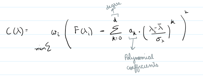
Methodology Overview:
- standardizes wave for numerical stability (polynomial fitting could be severely affected by large values)
- clips high percentile points based on flux
- sets a threshold (weights for points passing the threshold close to 1) – all weights [0,1]
- weighted polynomial fitting (so the brighter regions have more influence)
- this gives our continuum, then we just divid flux by continuum to get normalized flux
from scipy.signal import medfilt


def continuum_polynomial_weighted(wave, flux, deg=4, smooth=True):
    # scaling for numerical stability
    wave_scaled = (wave - wave.mean()) / wave.std()

    # initial smoothing using median filter
    if smooth:
        smoothed = medfilt(flux, kernel_size=5)#savgol_filter(medfilt(flux, 5), 51, 3)
    else:
        smoothed = flux

    # calculate weights based on residuals of smoothed spectrum
    residual = flux - smoothed
    mad = np.median(np.abs(residual - np.median(residual)))
    if mad < 1e-10:
        mad = 1e-3
    weights = np.exp(-((residual / (1.4826 * mad)) ** 2))  # Gaussian down-weighting
    weights = 1.0 / (1 + np.abs(flux - smoothed))
    # edge_fade = np.exp(-((wave - wave.mean()) / (wave.ptp() / 2))**2)
    # weights *= edge_fade

    coeffs = np.polyfit(wave_scaled, flux, deg=deg, w=weights)
    continuum = np.polyval(coeffs, wave_scaled)

    # clip to avoid div by zero or very small values and remove extreme high values
    continuum = np.clip(continuum, 1e-3, np.percentile(continuum, 99))
    # smooth the red tail
    continuum = smooth_tail(continuum, wave_scaled)

    norm = flux / continuum
    norm = np.clip(norm, 0.2, 3.0)

    return norm, continuum
- Pros: Soft masking avoids hard thresholds – more stable than hard masking – better fit than polynomial
- Cons: Still limited in flexibility compared to binned spline and savgols
Auto-Selected Continuum Method
Method: Applies all continuum methods, scores them based on smoothness, flatness, and curvature, and selects the best one automatically.
# Score = smoothness + 0.5 * flatness + 2.0 * clipping_penalty + 0.3 * curvature
best_method = min(scored, key=lambda x: x[3])
Methodology Overview:
- tries different techniques and picks up the best one
- scoring methodology is the key, to assess which one to pick, we first,
- measure how bumpy each continuum is by calculating smoothness which is a standard deviation from savgol (how bumpy)
- then we measure flatness i.e. if the normalized flux is centered around 1 (median = 1) (how centered)
- then we measure clip penalty – fraction of outliers or extreme points (outliers)
- then we measure curvature i.e.e how bendy the continuum is by calculating standard deviation of gradient (gradient stability)
- we combine all the above 4 metrics into a scre 1.0*smoothness + 0.5*flatness + 2.0*clip_penalty +0.3*curvature
- lower score indicates a better fit (smooth and more stable normalization)
# def score_method(cont):
#     smoothed = savgol_filter(cont, 101, 3)
#     smoothness = np.std(cont - smoothed)
#     flatness = np.abs(np.median(cont - 1.0))
#     return smoothness + 0.5 * flatness  # Weight toward smooth + ~1
from scipy.stats import wasserstein_distance

def score_method(norm, cont, wave):
    smoothed = savgol_filter(cont, 101, 3)
    smoothness = np.std(cont - smoothed) #checking jaggedness of continuum

    curvature = np.std(np.gradient(cont)) #fluctuations of continuum

    overshoot_penalty = np.mean(norm > 3.0) # penalize for too high peaks
    undershoot_penalty = np.mean(norm < 0.3)
    # clip_penalty = np.mean((norm > 5) | (norm < 0.2))
    clip_penalty = np.mean((norm > 2.5) | (norm < 0.5))  # out-of-bounds normalization

    flatness = np.abs(np.median(norm) - 1.0) #normalized spectrum must be centered around 1

    # line_contrast = np.std(norm[(norm < 1.0)])  # good absorption features
    absorption = norm[norm < 1.0]
    if len(absorption) > 10:
        line_contrast_penalty = 1.0 / (np.std(absorption) + 1e-6)  # larger std = deeper lines = better
    else:
        line_contrast_penalty = 5.0  # no lines = bad

    tail_mask = wave > 9000
    if np.sum(tail_mask) >= 3:
        tail_slope = np.mean(np.gradient(cont[tail_mask])) #checking slope of continuum in tail region
        tail_deviation = np.std(norm[tail_mask] - 1.0) #checking deviation from 1 in tail region
    else:
        tail_slope = 0
        tail_deviation = 0

    score = (
        1.0 * smoothness +
        0.5 * curvature +
        1.0 * flatness +
        2.0 * clip_penalty +
        2.0 * overshoot_penalty +
        1.5 * undershoot_penalty +
        1.0 * tail_deviation +
        0.5 * abs(tail_slope) +
        1.0 * line_contrast_penalty
    )

    score += wasserstein_distance(norm, np.ones_like(norm)) * 2.0
    return score

def auto_continuum_normalize(wave, flux, verbose=False, methods=None):
    if methods is None:
        methods = [
            "spline_wsavgol",
            "polynomial_weighted",
            "polynomial",
            "savgol"
        ]

    results = []

    # if flux.mean() < 100:
    #     methods = [m for m in methods if not m.startswith("polynomial")]


    for method in methods:
        try:
            if method == "spline_wsavgol":
                norm, cont = continuum_spline_wsavgol(wave, flux)
            elif method == "polynomial_weighted":
                norm, cont = continuum_polynomial_weighted(wave, flux)
            elif method == "polynomial":
                norm, cont = continuum_polynomial(wave, flux)
            elif method == "savgol":
                cont = savgol_filter(flux, window_length=151, polyorder=3, mode='interp')
                cont = np.clip(cont, 1e-5, None)
                norm = flux / cont
            else:
                continue  # Unknown method

            results.append((method, norm, cont))
            if verbose:
                print(f"{method} succeeded")

        except Exception as e:
            if verbose:
                print(f"{method} failed: {e}")

    if not results:
        raise RuntimeError("All continuum normalization methods failed.")


    scored = [(method, norm, cont, score_method(norm, cont, wave))
          for method, norm, cont in results]

    best_method, best_norm, best_cont, best_score = min(scored, key=lambda x: x[3])

    if verbose:
        print("Tried methods (with scores):")
        for method, _, _, score in scored:
            print(f" - {method}: {score:.4f}")
        print(f"Selected '{best_method}' with score {best_score:.4f}")

    return best_norm, best_cont, best_method
- Pros: Adaptable across diverse data qualities – selects best method for the data
- Cons: non standardized normalization – cant be used for NN, one continuum could be weighted polynomial and othe savgol – leading to inconsistency between data samples and features
For each technique, we visually inspected the normalized result to assess whether it retained key spectral features while flattening the continuum. This process helps guide preprocessing decisions for any spectral ML pipeline.
Conclusion
Spectrum normalization is not one size fits all. Your choice should reflect the data characteristics, application goals, and downstream models. Visual inspection is key, and automated scoring can help streamline the selection process.
The point of this normalization is to highlight spectral features like specific absorption or emission lines (super important for fingerprinting stars)
Even some of these fancier algorithms failed ‘catastrophically’ on some stars, based on what i saw so far, seems like spline with savgol might be our best bet — you should also modify the polynomial and weighted polynomial to atleast add a clipping so they don’t explode (because they did on some spectra).
I’ll add some comparisons for different types of stars and a side by side comparison with features extracted from manual inspection, so you can see what types of stars benefit from what type of normalization. Though for training ML models we would have to stick one methodology to maintain consistency.
I’ll follow up on that and any improvements in the scoring methodology for my auto function.
You can access this code on my github repo here