Code for this data extraction pipeline is available on my GitHub.
We live in such a dynamic world, the volatility and magnanimity of which we might not notice in our daily mundane lives, some of us glued to screen indoors be it rain or shine are even more disconnected to the reality outside.
I remember having this euphoric, scary, anxious, relieved feeling watching a lightning storm from inside my house, which believe it or not was popular enough that it got its own name in pop culture (google chrysalism meaning)
But out there, in the face of nature’s wrath, humans are insignificant. Over the years, we have advanced our methodologies, systems, and technology to better predict and manage events when nature refuses to cooperate with human development. Yet, despite our best efforts, there are events we can’t predict, can’t predict early enough, and can’t react to fast enough. The result is the inevitable damage to infrastructure, agriculture and even lives – be it human, animal, or plant – uprooting entire ecosystems at times!
We humans are insignificant in the face of one wild beast, much less the unprecedented fury of nature, and effective disaster management education, system and policy doesn’t even exist in all places. Be it wildfires, floods, earthquakes, tsunamis, volcanoes, landslides, avalanches, hurricanes – we hear something or the other in the news and once again get reminded of how powerless we still are in the face of a natural disaster.
I personally believe disaster management should not just be an academic exercise of a select few, but a humanitarian necessity, so, here lets start this flood prediction project as my humble attempt of trying something hoping the end result gives us all a better system in some aspect or even a better understanding that might help things down the line or someone very smart somewhere out there.
Also I want my time, and whatever I have learned, to be spent on something useful. This aligns with my life’s mission – trying to make and leave the Earth a better place while we’re on it, where life can prosper in harmony, we’ve come so far, unbelievable advances in science and technology over centuries of human effort and billions of years of biological and microbial effort to get us to the diversity and abundance of flora and fauna we see around us, including us, and so, we humans with our technology have a duty even if its just out of courtesy, protecting this planet called earth, for us and generations to come and letting life prosper throughout this universe. We owe it to all the earthen life that kept going, kept fighting, kept evolving billions of years.
We’re probably like the immune cell of earth’s ecosystem – a contract to do our part for the better of the system be it preventing harm, fighting asteroids or rebuilding civilizations – and i dont want to be a catastrophic neutrophil – no matter how passionate they are (and yes i’m currently reading immune by kurzgesagt)
I wanted to explore Physics Informed Neural Networks in Flood Prediction domain, but before we discuss models and methodologies – i’m currently looking into what exists in the space as well, first steps first lets get to know the data:
Here in my example – we’re extracting data for Ottawa-Gatineau 2019 floods, this is not necessarily the data i was aiming for my model – but i struggled finding decent global coverage for a lot of events and also a bit of lack of knowledge of terrain, urban and climatic influences, so to demonstrate the data acquisition we start at the home base.
Also to preface – I made use of GEE (Google Earth Engine) wherever possible – because it simplified the whole process of getting data.
When you’re working with multi modal data, this helps even more, instead of authenticating a million apis and learning their file systems and filtering and still getting massive chunks of data and frying your local machine trying to manually resample and interpolate the pixels- GEE lets you do that on ‘their’ server using a python GEE library – which has very very generous free tier for non commercial use. If you’re familiar with GIS tools you probably know a lot of tools like that (ArcGIS etc.) that do this but are quite slow and quite expensive.
Spatial Boundaries
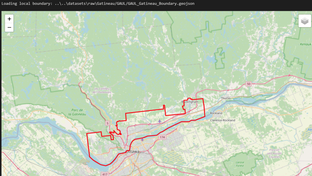
Before extracting the pixel data, we needs a spatial bounding box – to extract data for. For this, I used the Global Administrative Unit Layers (GAUL), compiled by the Food and Agriculture Organization (FAO).
- Level 0 – Country
- Level 1- States / Provinces
- Level 2 – Counties/Districts
Available through GEE (Google Earth Engine) – 2015 version
Earlier i was using GADM – GADM (Global Admin Boundaries) – using a filter on level 1 (states) and level 2 (districts/county) – but i realized GAUL seemed more reliable and accessible through GEE itself
Using GEE, I queried the Level 2 administrative boundary for Gatineau, Canada, and simplified the geometry to a 100m resolution. This reduces computational overhead while giving our arrays a precise mathematical boundary to clip against.
Here is how it looked:
Sentinel-1
If we want to observe a flood from space, first instinct might be to look at a photograph – data from an optical satellite like Sentinel-2. There is just one problem, floods happen during storms, and storms mean thick, impenetrable cloud cover. If we rely on optical data, we apparently will just get highly detailed pictures of white clouds lol
To actually see the water, we have to rely on different physics. We need what we call is Synthetic Aperture Radar (SAR) – which is basically things like microwaves instead of visible waves – we call it SAR because of the technology that makes this sort of scan possible.
To explain briefly – microwave wavelengths are like a x1000 more than light’s, to get an image resolution of say 10m (sentinel satellite’s resolution) from earth’s orbit like 700km high – would require a 4km antennae or something – the technological workaround is – the satellite has a number of antennae – and they send 1000s of microwaves and since they’re microwaves they can pass through the clouds and they get reflected on the surface and are recorded, corrected for doppler shifts and combined using Fourier transforms.
in our case, operated by the European Space Agency (ESA), Sentinel-1 is a polar-orbiting satellite that actively sends microwave pulses down to Earth. Because microwaves have much longer wavelengths than visible light, they pass right through clouds and heavy rain. When these pulses hit the ground, they scatter, and the satellite measures the “backscatter” that returns.
Here is where the physics of fluids and flat surfaces comes in: water acts like a flat mirror to microwaves. When the radar hits a flooded area, the energy bounces away from the satellite, resulting in a very low backscatter signal. In our data, floodwaters appear distinctly dark.
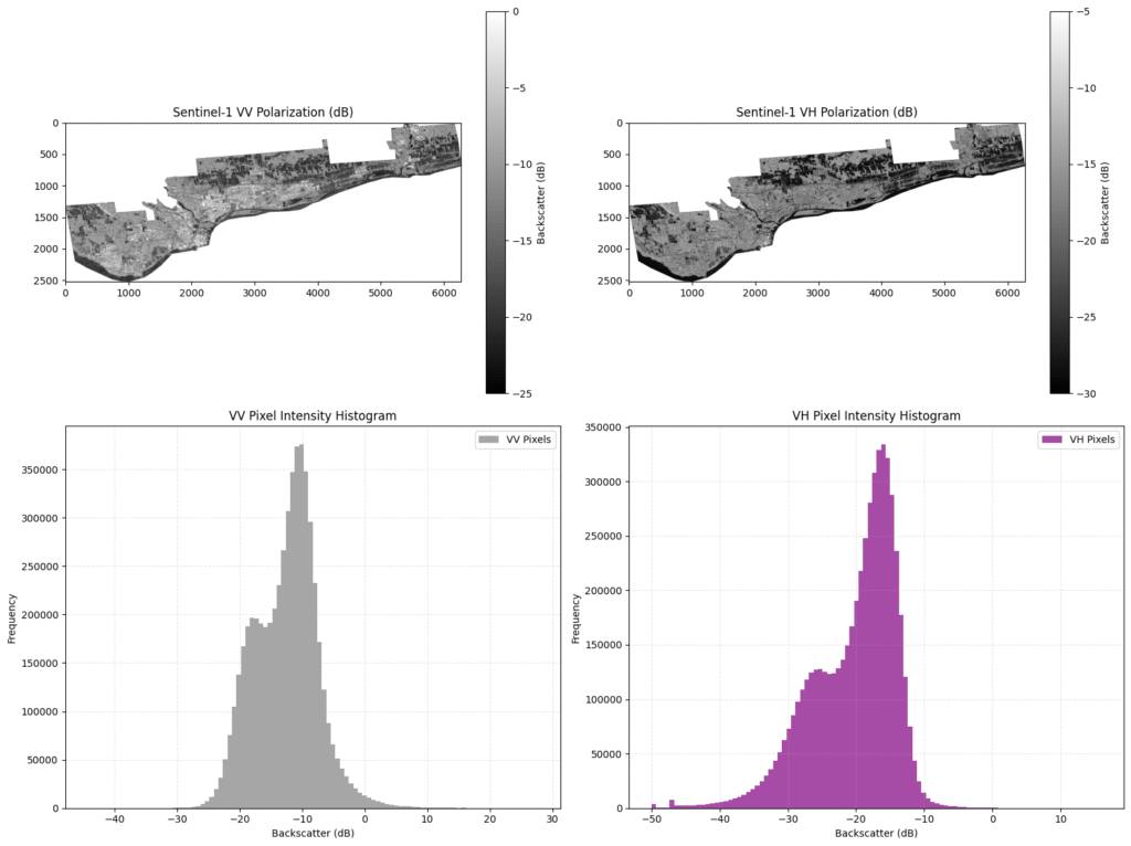
For this project, I pulled Sentinel-1 Interferometric Wide (IW) swath data using two specific polarizations:
- VV (Vertical Transmit, Vertical Receive): Highly sensitive to surface roughness, making it our primary tool for detecting open water because of surface scattering, open floodwaters act like a flat mirror, the vertical radar waves bounce away from the satellite, making the water appear distinctly dark. Looking at the VV histogram, we see a clean, bimodal (two-peak) distribution. The distinct peak on the left (lower dB values) represents the water, while the larger peak on the right represents the rougher, brighter land.
- VH (Vertical Transmit, Horizontal Receive): Sensitive to volume scattering, which helps us distinguish between flooded vegetation and clean open water.
it is noticeably noisier and darker overall because VH relies on depolarization the radar wave must hit a complex, 3D structure (like a tree canopy or a building) and bounce around inside it to return a horizontal signal. Its histograms different as well, the entire distribution is shifted left toward lower decibel ranges, and the split between water and land can be much more blurrier.
The Environmental Stack
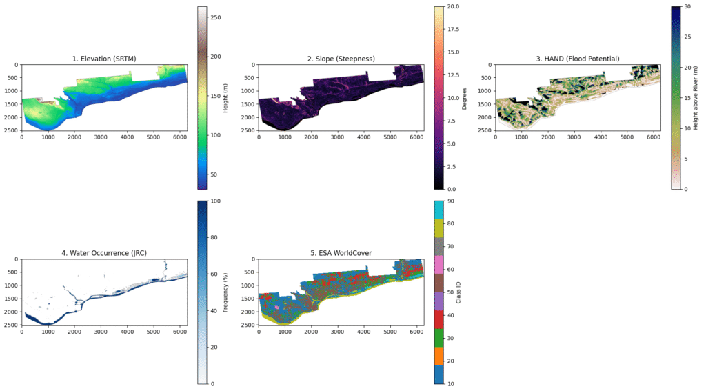
To predict a flood, the model needs to understand the landscape just as well as the water does. Water flows downhill, pools in basins, and absorbs differently depending on the ground beneath it. To capture this physical reality, I built a single, multi-dimensional tensor out of four distinct environmental layers: a Digital Elevation Model (DEM), Height Above Nearest Drainage (HAND), JRC historical surface water, and ESA WorldCover and this is where GEE shines
Elevation
Digital Elevation Model (DEM): Sourced from NASA’s SRTM, giving us absolute height. Water flows downhill, making elevation the most fundamental constraint.
Shuttle Radar Topography Mission (SRTM) was a 2000 NASA mission with the shuttle Endeavour mapping 80% of the earth, the GEE dataset we used here is – USGS/SRTMGL1_003
Slope
Derived from the DEM, this tells the model about terrain steepness. Steep slopes mean rapid runoff and flat areas mean pooling
Relative Elevation
Height Above Nearest Drainage (HAND): Relative elevation is critical. HAND normalizes topography based on the local drainage network, directly highlighting low lying floodplains. THE GEE Dataset is – gena/GlobalHAND/30m/hand-1000 – derived from DEM so also the year 2000
Water Bodies
JRC Global Surface Water (Occurrence): To predict a flood, we must know what isn’t a flood. We use this historical map to mask out permanent water bodies (like existing rivers) so the model learns to identify anomalous flooding.
The Joint Research Centre is a European initiative compiling (1984-present) ~35 yr summary and can be accessed in GEE through JRC/GSW1_4/GlobalSurfaceWater
Land Use
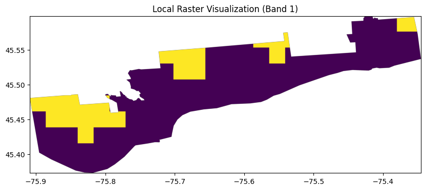
ESA WorldCover: Finally, we classify the surface material (urban, agriculture, forest) to implicitly account for different fluid friction and absorption coefficients. Its a global map by European Space Agency using Sentinel1 and Sentinel2 data and can be acccessed in GEE through ESA/WorldCover/v200 – which is a 2021 version
I could do all that with just this:
def get_environment_stack_gee(roi):
    dem = ee.Image("USGS/SRTMGL1_003").clip(roi).rename('elevation')
    slope = ee.Terrain.slope(dem).rename('slope')

    hand = ee.Image("users/gena/GlobalHAND/30m/hand-1000").clip(roi).rename('hand')

    water_occ = ee.Image("JRC/GSW1_4/GlobalSurfaceWater").select('occurrence').clip(roi).rename('water_occ')

    landcover = ee.ImageCollection("ESA/WorldCover/v200").first().clip(roi).rename('landcover')

    # Stack and resample to 10m to match the S1 resolution we got
    return ee.Image.cat([dem, slope, hand, water_occ, landcover]).float()

def export_env_stack(roi, region_name, clean_region_name):
    stack = get_environment_stack_gee(roi)

    task = ee.batch.Export.image.toDrive(
        image=stack,
        description=f"{clean_region_name}_Env_Stack",
        folder=f"Flood_Project_Data",
        fileNamePrefix=f"ENV_{clean_region_name}_env_stack",
        region=roi,
        scale=CONFIG['PARAMS']['s1_resolution'],
        crs='EPSG:4326',
        maxPixels=1e9
    )
    task.start()
print(f"Environmental stack export started for {clean_region_name}")This looks somewhat like:
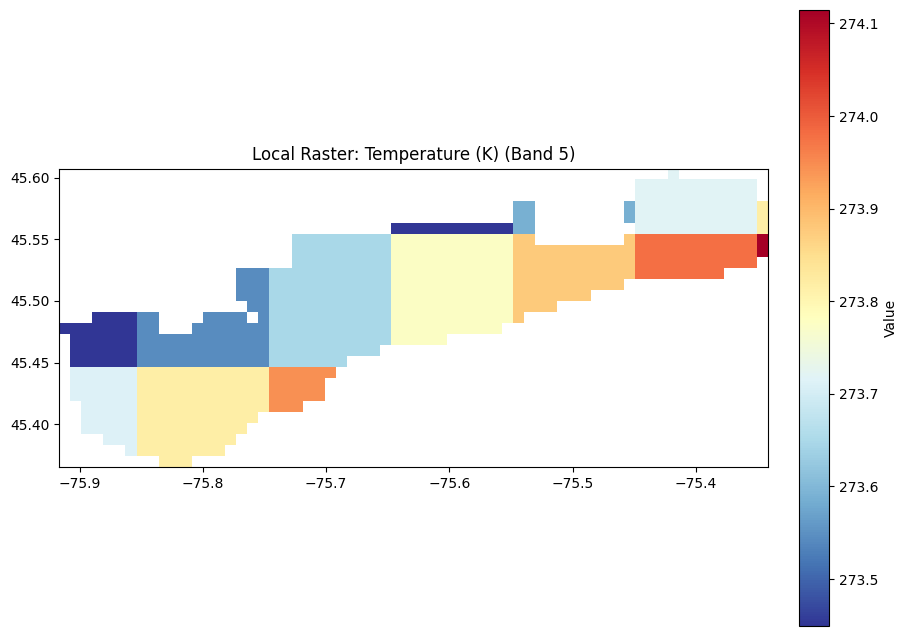
The Forcing Function – The Weather Data
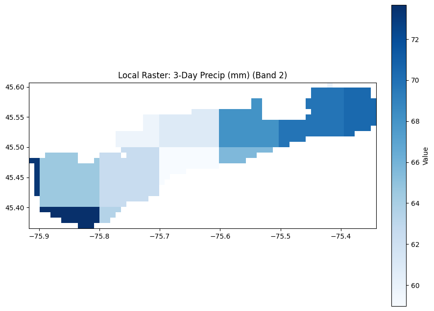
A landscape doesn’t flood itself, it requires an atmospheric forcing function. To give the model the cause-and-effect relationship, I extracted 1km-resolution weather grids covering the weeks leading up to and during the flood. By ingesting daily precipitation (how much water is falling) and temperature (critical for identifying spring snowmelt in the Canadian context at least) – also temperature is usually* most indicative of a lot of weather anomalies, seasonality and patterns
Weather
For temperature and weather in general the gold standard in ML is ERA5 🙂
its ECMWF’s historic reanalysis dataset – the best part is the general consistency, variables and lookback (1940 to present!) – not that we are planning to use all the variables and that time range and of course other datasets exist and other models might be more accurate for predictions than HRES forecasts for your specific locale and some weather patterns but there’re pros and cons, if it helps make the case, google trained Graphcast on ERA5 as well. (But yes please await my weather datasets blog where i dive into weather data in more detail!)
ERA5 resolution is ~30km
Other
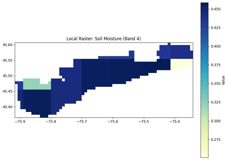
We also use SMAP (Soil Moisture Active Passive) to have an estimate of moisture content in the soil, this is a global dataset that estimates the moisture content in top 5cm of soil using microwaves (SMOS, GLDAS are some other options as well)
GPM IMERG (Global Precipitation Measurement) which is global – every 30 min – radar + microwave with a 10km spatial res (way coarser than S1’s 10m.
alternative – CHIRPS (long term res), NEXRAD, MRMS (only North America)
Hydrography
Global Hydrography (MERIT Hydro) – While a DEM tells us the elevation of a single point, water dynamics require us to know how those points connect. For this, the hydrology community relies on datasets like MERIT Hydro. It explicitly maps flow direction and flow accumulation. It tells the model not just that water flows downhill, but which river channel it will eventually end up in. It has about 90m resolution, there are other alternatives like NHDPlus but that primarily covers the States
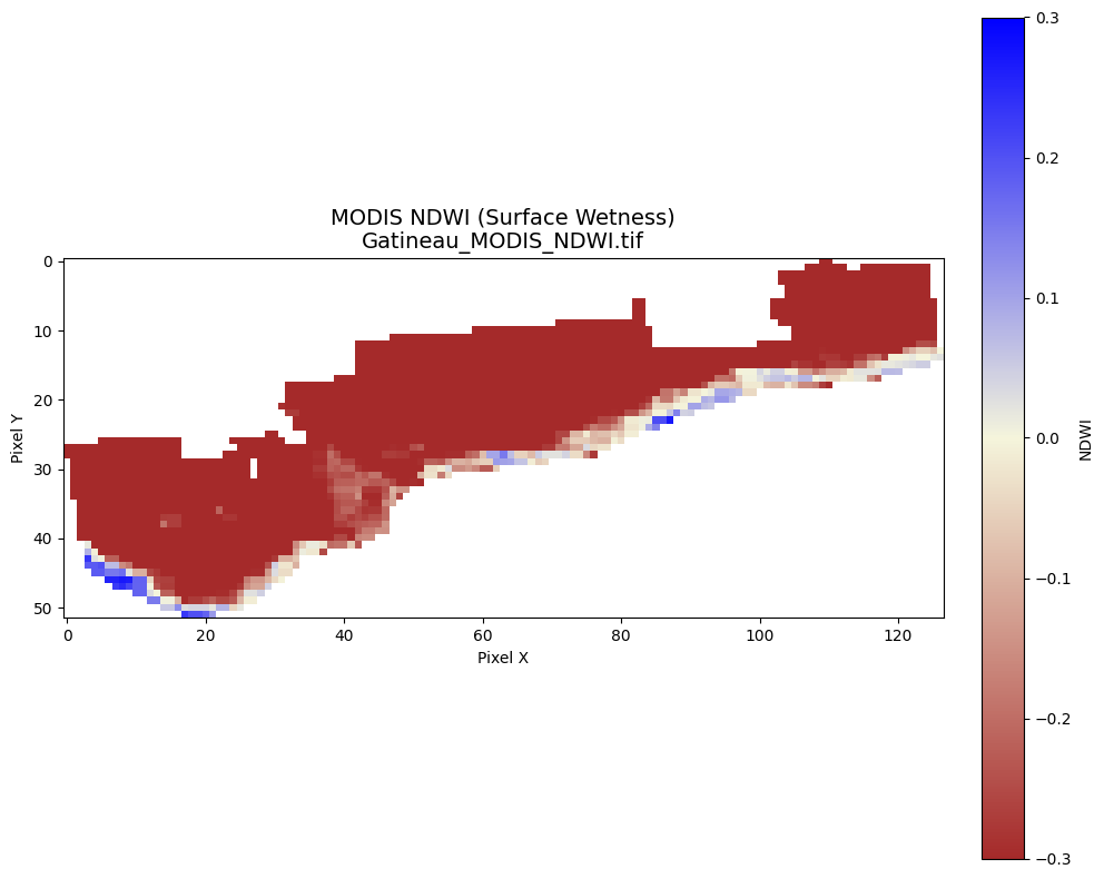
Optional – MODIS (The Optical Backup)
While Sentinel-1 SAR is our primary “see-through-clouds” tool, NASA’s MODIS (Moderate Resolution Imaging Spectroradiometer) aboard the Terra and Aqua satellites remains a workhorse of Earth Observation. MODIS images the entire Earth every 1 to 2 days. While it is blinded by the storm clouds during the peak of a disaster, its high temporal frequency makes it incredible for tracking the long term duration of a flood once the skies clear, serving as a powerful secondary validation layer for our model’s predictions. It is a bit coarse with 1 pixel potentially corresponding to 250-500m
The Operational Ecosystem – EMS, GFM, GloFAS
These are some benchmarks / potential labels if we were to train a prediction model
- Copernicus EMS (Emergency Management Service): Run by the European Union, EMS is the rapid-response paramedic of the satellite world. When a disaster strikes, authorized users (like civil protection agencies) can trigger EMS. They rapidly task satellites to acquire imagery and produce standardized flood extent and damage assessment maps within hours to guide rescue teams on the ground.
this is a gold label dataset – high resolution manually verified labels
The challenge is – that it only covers selected major disasters – it has to be specificially requested by the government
also, it could be based on imagery from multiple satellites - GFM (Global Flood Monitoring): Part of the Copernicus operational suite, GFM is an automated system that continuously ingests every single incoming Sentinel-1 SAR image globally. It runs ensemble algorithms to detect flooded pixels in near real-time, providing a constant, automated heartbeat of global water anomalies.
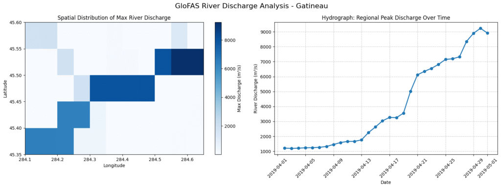
The good part is – its 24/7, covers the entire globe, runs on sentinel-1 but an important consideration is – GFM itself is an output of another model - GloFAS (Global Flood Awareness System): While EMS and GFM observe the present, GloFAS predicts the future. It is a hydrological forecasting system that takes weather forecasts and routes them through massive river network models. It can issue early warnings of high river flows days or even weeks in advance.
Bringing it Together
This enables us to essentially construct a multi-modal digital twin of the region during a moment of crisis, think about what sits inside these tensors:
We have the absolute constraints of the Earth’s surface (DEM, Slope, HAND), the historical memory of the rivers (JRC, MERIT Hydro), the physical friction of the landscape (ESA WorldCover), the atmospheric fury that caused the event (Weather data), and the exact microwave reflection of the floodwaters as seen from 700 kilometers in space (Sentinel-1 SAR.
But right now, this data is raw. The Sentinel-1 SAR imagery is riddled with radar speckle noise, the weather data needs to be temporally aligned with satellite flyovers, and our environmental stacks need to be perfectly normalized so our neural network doesn’t mathematically prioritize a 1000-meter elevation over a 10-millimeter rainfall
We now have the physical ground truth. In Part II, we will look at how to clean this data, process the signal noise, and prep the tensors to feed our predictive model.
Right now what i think next TODOs are:
- Clean the SAR speckle noise (Lee/Refined Lee filters?)
- Ground Truth – Otsu’s thresholding to the VV band to create our binary “Ground Truth” water masks – compare with GFM
- Align and normalize the spatial temporal tensors so they are ready to be ingested by a PyTorch DataLoader
- Once we have created and integrated data prep pipeline – maybe we will verify with another well known event also mapped by EMS
Code for this data extraction pipeline is available on my GitHub.