Bucketing and discretization is important step in any algorithmic training or analysis, today we focus on the ways we can map the continuous spherical surface of Earth into manageable buckets. Why exactly we do this? to index different locations on earth to allow for fast geospatial queries, joins and aggregations. There are three popular geo indexing systems – Geohash, Uber’s H3 and Google’s S2, all let you map (lat, lon) -> a cell id, but they differ in what surface they discretize and therefore what kinds of distortion they introduce
Geohash
Divides the map into a standard grid, but the physical size of the grid shrinks at the poles
Structure
- Rectangular cells
- Recursive subdivision in lat/lon space
Distortion
- Uniform in degrees (not in meters)
- Physical width of cells shrinks toward the poles
Indexing
- uses a Z-order curve for indexing
- outputs a base-32 string
- prefix matching – same prefix – closer – allows spatial clustering by text match
H3
Maps the Earth to an icosahedron (20 faces) covered in hexagons, developed Uber
Structure
- Discretize the sphere using an icosahedron and mostly hexagonal cells
- requires a small number of pentagons to fil in the gaps
- mostly uniform cells – great for grid math (neighbors, rings, disks)
- distance from center is identical
Distortion
- Distortion exists (as its on a sphere), but is spread relatively evenly
Indexing
- Uses an aperture 7 system (subdividing each cell into 7 smaller parts
- Hexagons give strong neighborhood properties (k-rings, local adjacency)
S2
Maps the earth to a cube, then projects it onto a sphere, subdivide cube faces, then project back to the sphere, developed by Google
Structure
- Each face is recursively subdivided into four child cells (a quadtree), resulting in quadrilateral-ish cells on the sphere
Distortion
- Bounded and well behaved globally, with better behavior near the poles compared to planar lat-lon grids
Indexing
- uses a Hilbert space curve
- Great for hierarchy with predictable parent/child relationships
- very fast because maps to 64bit integers
Size and Precision
Geohash
Resolution Levels
1 to 12 (12 characters total)
Hierarchy: base 32 string – every character is 5 bit worth of precision which means exponential scaling. Z curve indexing to divide further on each level
Level 1 starts with, 8 columns (ie 360/8 = 45 degree lon), 4 rows (ie 180/4 = 45 degree lat) = 5000x5000km blocks
Neighborhood Geometry: In a rectangular grid, the distance to vertical and horizontal neighbors is 1, but the distance to diagonal neighbors is 2^(1/2)
Precision Breakdown:
- Level 4 (Metropolitan): ~39 km
- Level 5 (City): ~5 km
- Level 6 (Neighborhood): ~1.2 km
- Level 12 (Maximum Precision): ~3.7 cm by 1.8 cm
H3
Resolution Levels
0 to 15
Hierarchy: Because hexagons cannot be perfectly subdivided into smaller hexagons (aperture 7 system – hexagons +pentagons), H3’s sub-hierarchy is not perfectly contained (child cells slightly overlap parent boundaries)
Neighborhood Geometry: The distance from the center of a hexagon to all six of its adjacent neighbors is exactly equal. This makes it mathematically superior for radial calculations and smoothing
Precision Breakdown:
- Level 0 (Continental): ~1100 km edge length
- Level 3 (State): ~60 km
- Level 5 (City): ~8.5 km
- Level 7 (Neighborhood): ~1.2 km
- Level 15 (Maximum Precision): ~0.5 m
S2
Resolution Levels
0 to 30
Hierarchy: A perfect quadtree. Every parent cell is mathematically subdivided into exactly 4 child cells, with zero edge overlap
projects earth to cube – cube is level 0 (cell at 0 = 1/6 earth)
Neighborhood Geometry: Cells are indexed using a continuous Hilbert curve, which avoids the spatial “jumps” seen in the Geohash Z-curve. Because S2 maps directly to 64-bit integers, computational operations are incredibly fast
Precision Breakdown:
- Level 0 (Continental): ~10,000 km edge length
- Level 4 (Country): ~576 km
- Level 10 (City): ~9 km
- Level 13 (Neighborhood): ~1 km
- Level 20 (House): ~8 m
- Level 24 (Surveying): ~55 cm
- Level 30 (Maximum Precision): ~0.9 cm
Grid Cells
To see how these indexing systems behave in practice, let’s look at a specific coordinate in Ottawa (Lat: 45.428, Lon: -75.718) and map it to a “City” resolution across all three systems.
We choose the following resolution / level for each grid system:
"city": {"geohash": 5, "h3": 6, "s2": 11}which ranges from 16 – 40 km2 (City Ward / Large District)
While Geohash, H3, and S2 all have a scale that conceptually maps to a “City District” their actual geometric footprints vary wildly:
Size
- Geohash (Precision 5)
- Token: f244k (Parent: f244)
- Centroid: 45.417480, -75.739746
- Dimensions: 3433.86m x 4891.99m
- Estimated Area: ~16.8 million m² (16.8 km²)
- H3 (Resolution 6)
- Token: 862b83b1fffffff (Parent: 852b83b3fffffff)
- Centroid: 45.419360, -75.762752
- Edge Length: 3950.16m
- Estimated Area: ~39.3 million m² (39.3 km²)
- S2 (Level 11)
- Token: 4cce04c (Parent: 4cce05)
- Centroid: 45.443463, -75.710880
- Edge Length: 3828.80m
- Estimated Area: ~16.1 million m² (16.1 km²)
Quantization
Quantization error – cell centroid distance – If we are putting a cell around a lat lon – how far is the cell center from the lat lon, we compare this on the smallest scale:
- Geohash (Precision 12)
- Token: f244kvzv68zp (Parent: f244kvzv68z)
- Centroid: 45.428000, -75.718000
- Dimensions: 0.03m x 0.02m
- Estimated Area: ~0.0005 m²
- H3 (Resolution 15)
- Token: 8f2b83b1d90b96d (Parent: 8e2b83b1d90b96f)
- Centroid: 45.427996, -75.718002
- Edge Length: 0.6174m
- Estimated Area: ~0.9731 m²
- S2 (Level 30)
- Token: 4cce04f4d08605cd (Parent: 4cce04f4d08605cc)
- Centroid: 45.428000, -75.718000
- Edge Length: 0.0073m
- Estimated Area: ~0.0001 m²
For the given Lat: 45.428, Lon: -75.718, we’ve computed the distance of the point from the centroid (haversine distance – the details of which you can read in the next section)
the smallest possible quantization error:
Geohash(12) Off-Center Distance: 0.01 meters
H3 (15) Off-Center Distance: 0.52 meters
S2(30) Off-Center Distance: 0.00 meters
city level quantization error (for the cell size displayed in the image):
Geohash(5) Off-Center Distance: 2061.21 meters
H3 (6) Off-Center Distance: 3622.33 meters
S2(11) Off-Center Distance: 1806.92 meters
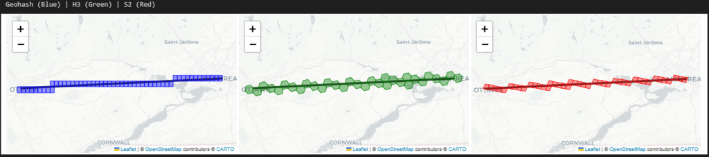
Notice the massive discrepancy in area. At the city tier, S2 and Geohash yield a similarly sized bounding box (~16 sq km), but H3’s hexagonal resolution jumps to nearly 40 sq km. Furthermore, the centroids of these cells do not perfectly align with the target coordinate. This highlights a crucial rule for geospatial engineering: you cannot blindly swap indexing systems and expect a 1:1 mapping. You must tailor the resolution level to the specific precision required by your dataset.
Distance
Planar
Flat map distance, given latitude and longitude of two points, we employ an equirectangular projection and calculate Euclidean distance.
Point 1: $(\phi_1, \lambda_1)$ , Point 2: $(\phi_2, \lambda_2)$
$\phi$ = latitude (radians), $\lambda$ = longitude (radians), $R$ = Earth radius
Reference point $(\phi_0, \lambda_0)$
Projection Center (reduce distortion):
$\phi_0 = \frac{\phi_1 + \phi_2}{2}$
$\lambda_0 = \frac{\lambda_1 + \lambda_2}{2}$
Equirectangular Projection :
east-west displacement in meters
$x = R \cdot (\lambda – \lambda_0) \cdot \cos(\phi_0)$
$\cos(\phi_0)$ term corrects for the fact that lines of longitude
get closer together toward the poles
north-south displacement in meters
$y = R \cdot (\phi – \phi_0)$
Euclidean Distance in Projected Space (m) :
$d = \sqrt{(x_2 – x_1)^2 + (y_2 – y_1)^2}$
Geodesic
Because the earth is curved, to find distance between two points specified with a latitude or longitude, we employ the haversine formula.
Point 1: $(\phi_1, \lambda_1)$ , Point 2: $(\phi_2, \lambda_2)$
$\phi$ = latitude (radians), $\lambda$ = longitude (radians), $R$ = Earth radius
$\Delta \phi = \phi_2 – \phi_1$, $\Delta \lambda = \lambda_2 – \lambda_1$
Haversine:
$a = \sin^2\left(\frac{\Delta \phi}{2}\right)+ \cos(\phi_1)\cos(\phi_2)\sin^2\left(\frac{\Delta \lambda}{2}\right)$
Angular Distance:
$c = 2 \cdot \arctan2\left(\sqrt{a}, \sqrt{1-a}\right)$
Final Distance:
$d = R \cdot c$
For a collection of points as follows:
test_pairs = {
    "local": [(45.428, -75.718), (45.47, -75.70)], #(Ottawa ~5km)
    "regional": [(45.428, -75.718), (45.5017, -73.5673)], #(Ottawa–Montreal)
    "cross_country": [(45.428, -75.718), (49.2827, -123.1207)], #(Ottawa–Vancouver)
    "equator": [(0.0, 0.0), (0.0, 10.0)], #(0°, 0° - 0°, 10°)
    "poles": [(70.0, 0.0), (70.0, 60.0)], #(70°, 0° - 70°, 60°)
}

levels = {
    # "neighborhood":{"geohash": 6,"h3": 7,"s2": 13},
    "smallest":{"geohash": 12, "h3": 15, "s2": 30},
    "largest":{"geohash": 1, "h3": 0, "s2": 0}, # geohash 0 is the whole world
    "state": {"geohash": 3, "h3": 2, "s2": 6}, # 100,000+ km2 (State / Province Level)
    "metro": {"geohash": 4, "h3": 4, "s2": 8}, # 500+ km2 (Wide Metro Area / County Level)
    # "city" :{"geohash": 5, "h3": 5, "s2": 10},
    "city": {"geohash": 5, "h3": 6, "s2": 11}, #16 - 40 km2 (City Ward / Large District)
    "neighborhood": {"geohash": 6, "h3": 7, "s2": 12}, #5 km2 (Neighborhood),
    "sentinel_scale": {"geohash": 8, "h3": 12, "s2": 20} #10m approx
}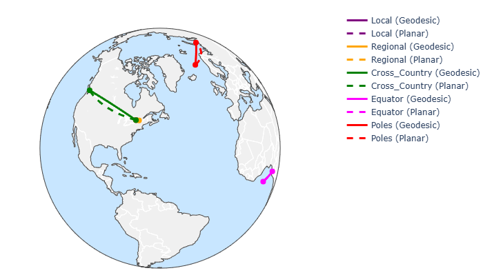
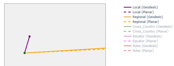
we see the geodesic and planar distance are noticeably different on large scales because of earth’s curvature
Now lets compare the error between haversine distance for the actual points vs the cell centroids:
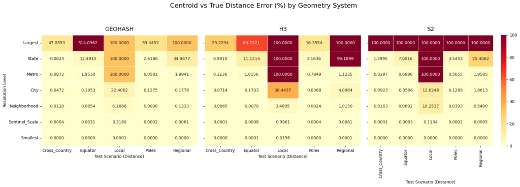
The “Local” Distance Anomaly: If you look at the “Local” test scenario (a distance of roughly 5 km) across all three systems, the error hits exactly 100.0000% at the “State” and “Largest” levels. This happens because the physical distance being measured is vastly smaller than the cell itself. If both points fall into the exact same massive cell, the calculated centroid distance is 0, resulting in a 100% error. This is a vital reminder: never use a spatial index resolution that is physically larger than the phenomena you are trying to measure.
Geohash’s Equator Extreme: At the “Largest” resolution level, Geohash struggles massively at the Equator, showing a staggering 314.0962% error. By comparison, H3 at the Equator for the same level shows a 64.7221% error. Geohash’s rectangular planar projection simply cannot handle extreme longitudinal distances reliably at a low resolution.
S2’s Rigorous Bounding: Look at S2’s “Largest” row: it hits a flat 100.0000% error across all scenarios. Because S2 Level 0 cells cover exactly one-sixth of the Earth’s surface, almost all of our test pairs snapped to the same massive cell centroid. However, as soon as you step down to the “Metro” and “City” levels, S2’s errors drop rapidly and consistently.
Convergence at the Sentinel Scale: By the time we reach the “Sentinel_Scale” (roughly 10-meter resolution, perfect for satellite imagery) and the “Smallest” scale, all three systems converge to near 0.0000% error, regardless of whether you are tracking a cross-country flight or a localized grid outage
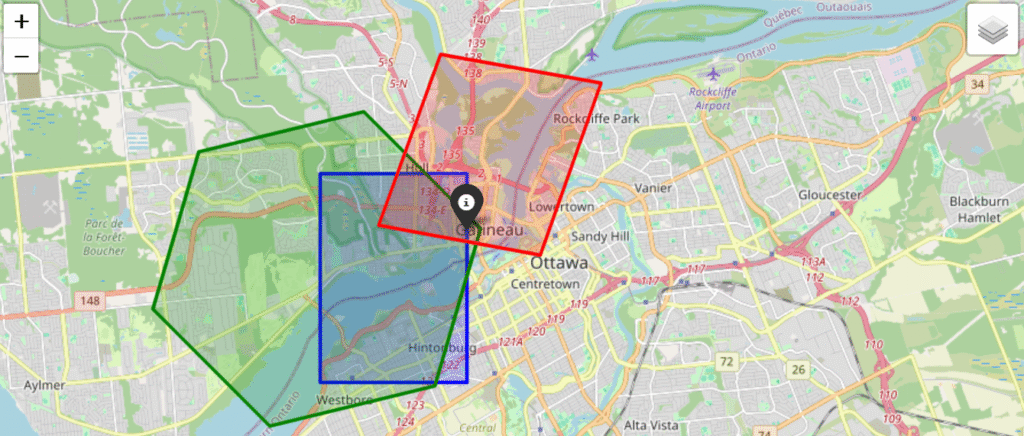
The following is how the ‘city’ level cells look like over a regional distance
Intersect
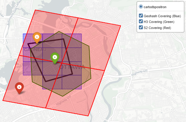
By intersect what we mean is geofencing and point in polygon problem, in most of geospatial problems, we will constantly be checking if telemetry coordinates fall within a specific boundary, and for that we can either do the exact mathematical calculation (which is computationally expensive at scale) or check if the point belongs to a pre computed set of grid cells (which is blazing fast but introduces edge-case errors)
When determining if a point falls inside a complex polygon, we use these test cases (firmly inside the polygon, riding the borderline, and just outside) and compare the exact geometric calculation (using the Shapely library) against native grid set lookups across Geohash, H3, and S2 at the “Neighborhood/City” scale.
geofence_poly = [ #downtown ottawa - bounding box
    [45.430, -75.715],
    [45.432, -75.695],
    [45.418, -75.690],
    [45.415, -75.705],
    [45.430, -75.715]
]

test_points = {
    "Inside": (45.422, -75.700),
    "Borderline": (45.430, -75.710),
    "Outside": (45.410, -75.720)
}| Point_Type | Lat_Lon | Exact_Contains | GEOHASH_In_Set | H3_In_Set | S2_In_Set | GEOHASH_Intersects | H3_Intersects | S2_Intersects | Exact_Time_ms | GEOHASH_Set_Time_ms | H3_Set_Time_ms | S2_Set_Time_ms | GEOHASH_Intersect_Time_ms | H3_Intersect_Time_ms | S2_Intersect_Time_ms | |
|---|---|---|---|---|---|---|---|---|---|---|---|---|---|---|---|---|
| 0 | Inside | 45.422, -75.7 | True | True | True | True | True | True | True | 0.0193 | 0.0059 | 0.0031 | 0.0143 | 0.0065 | 0.0149 | 0.0054 |
| 1 | Borderline | 45.43, -75.71 | True | True | False | True | True | True | True | 0.0053 | 0.0054 | 0.0018 | 0.0142 | 0.0046 | 0.0063 | 0.0050 |
| 2 | Outside | 45.41, -75.72 | False | False | False | True | False | False | True | 0.0500 | 0.0065 | 0.0030 | 0.0160 | 0.0064 | 0.0068 | 0.0082 |
Where In Set is a still a mathematical intersects (using shapely) for the cell polygon and intersects is the the grid systems native intersect function.
The Inside Point: All three systems, as well as the exact calculation, correctly identified that the point was inside the polygon. No surprises here.
The Borderline Point: The exact math confirmed the point was inside. Geohash and S2 successfully flagged it via set lookup. However, H3’s native set lookup returned False. Because hexagons don’t perfectly conform to sharp, straight polygon edges, the H3 polyfill algorithm left a slight gap at the border, resulting in a false negative.
The Outside Point: The exact math correctly flagged the point as outside. Geohash and H3 agreed. However, S2 returned True for both the set lookup and dynamic intersection. Because the S2 cell at this specific resolution level was large enough to overlap the polygon boundary while also swallowing the outside point, it yielded a false positive.
Now you ask if grids introduce false positives and negatives, why use them at all? Speed!
- Exact Geometry (Shapely): Ranged from 0.0053 ms to 0.0500 ms. Exact math is highly variable because the computational cost increases depending on how complex the polygon is and where the point lies relative to its edges. This was a simple bounding box, but geo polygons can be and usually are very detailed
- Geohash Set Lookup: Hovered around ~0.0054 to 0.0065 ms.
- S2 Set Lookup: Ranged from ~0.0142 to 0.0160 ms.
- H3 Set Lookup: Blew the competition away at 0.0018 to 0.0031 ms
(and we can always solve for accuracy by adjusting resolution and/or employing hierarchal checks)
Neighborhood
In geospatial analytics, we rarely look at a single cell in isolation.
Not just optimal drive time solutions but even in Earth Observation problems we apply smoothing filters, calculate local density, or model the spread of phenomena (like a flood or a signal footprint) by radiating outward. This requires pulling a cell’s immediate neighbors.
Based on our analysis at the “Neighborhood” scale (roughly 1 to 5 km²), here is how Geohash, H3, and S2 handle spatial adjacency
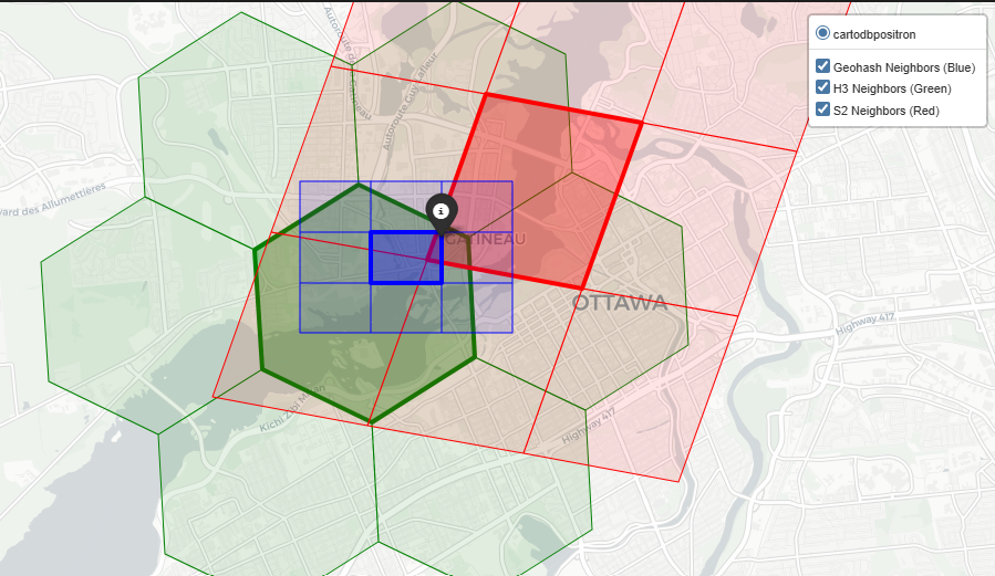
Geohash
Geohash is computationally simple, but library support for adjacency can be lacking. For instance, the pygeohash library does not have an inherent function to fetch neighbors.
- The Method: To find neighbors, we had to manually calculate the latitude and longitude error margins (the dimensions of the cell) and step outward to create a 3×3 grid around the center token
- The Result: You get 8 neighbors (sharing edges and corners). However, because Geohash relies on a Z-order curve, cells that are physically adjacent might have wildly different string prefixes, making database range queries for neighbors highly inefficient
H3
Uber’s H3 system was made for this. Hexagons are the gold standard for neighborhood traversal because the distance from the center of a cell to all of its neighbors is identical.
- The Method: H3 uses a built-in
grid_disk(center, k=1)function, which efficiently returns the center cell plus its immediate ring of neighbors
- The Result: You get exactly 6 perfect neighbors. If you are building a Convolutional Neural Network (CNN) or a Graph Neural Network (GNN) that requires pooling data from adjacent spatial regions, H3’s uniform
k-ringexpansion makes the math incredibly clean
S2
S2 handles neighbors robustly, leveraging its 64-bit integer indexing and Hilbert curve.
- The Method: S2 provides a native
get_all_neighbors(level)function
- The Result: It returns 8 neighbors in total: 4 edge-sharing neighbors and 4 vertex-sharing (corner) neighbors. Because S2 avoids the severe spatial jumps of Geohash’s Z-curve, fetching these neighbors is computationally fast, though the variable distance to corner neighbors makes it slightly less ideal for radial smoothing than H3
Hierarchy & Coverage
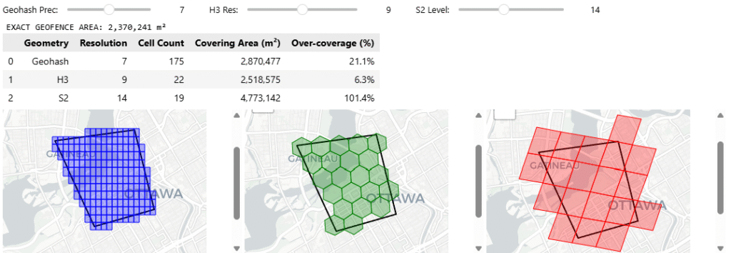
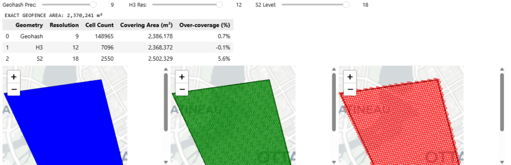
we’ve already established how these systems group cells (hierarchy) and how they fill a shape (coverage) are fundamentally different, now we tackle on a problem of indexing a geographic boundary – to retrieve data inside, here we see how at different hierarchies and resolutions, different grid cells cover a geographic area
Geohash
Hierarchy: Geohash’s hierarchy is incredibly simple for databases. If your cell is f244k, its parent is f244. You just chop off the last character. It is fast for text-based NoSQL scans, but because of the Z-curve, a parent cell might contain child cells that are physically distorted or seemingly disjointed
Coverage: Geohash lacks a native, sophisticated region coverer in most standard Python libraries. To cover a polygon, we had to manually generate a bounding box and iterate through coordinates. This brute force method almost always results in high over coverage at the polygon’s edges because rectangular cells do not hug diagonal borders well
H3
Hierarchy: H3 uses an “aperture 7” hierarchy, meaning one parent hexagon roughly contains seven child hexagons. However, geometry dictates that hexagons cannot be perfectly subdivided into smaller hexagons. This means H3’s hierarchy is not perfectly nested, child cells will slightly overlap the boundaries of their parent
Coverage: H3 offers a native polygon_to_cells polyfill function. Because hexagons approximate organic, curved, and diagonal shapes much better than rectangles, H3 provides a very tight footprint with minimal over-coverage, saving compute on downstream queries
S2
Hierarchy: S2 is mathematically flawless here. It uses a pure quadtree hierarchy where exactly 4 child cells fit perfectly inside 1 parent cell with zero boundary overlap. For hierarchical data aggregations, S2 is vastly superior
Coverage: S2 is purpose-built for this. It has a native RegionCoverer() class that allows you to specify a min_level, max_level, and even a maximum cell count. It mixes large parent cells in the center of the polygon and small child cells at the complex borders, optimizing both accuracy and database storage
You can access the code here github
Leave a Reply