We categorize stars into different types based on attributes like Luminosity, Temperature and size – but how do we define it and measure it, lets discuss briefly
Brightness
One of the most important attributes of stars is their brightness, how bright or dim they are and how they appear to us. It is a measure of the electromagnetic waves that we receive and is usually limited to a particular band in the electromagnetic spectrum (visible or any other specific filter we use in our telescopes). Brightness is also referred to as Flux.
We quantify the brightness of a star in units of Magnitude
Brightness (apparent) refers to how bright the star appears to us and intrinsic brightness (Luminosity) is how bright the star actually is. We don’t get to observe all the light from the star for multiple reasons:
– For one the photon’s wavelength stretches over large distances – light redshifts, falls to infrared, microwaves to radiowaves (doppler redshift, cosmological redshift, gravitational redshift)
– Interstellar dust and gases obstructing the path of light
– Atmospheric turbulence, moisture, dusts and gases
– The wavelength of the filter we use to observe
Luminosity
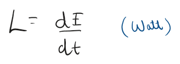
Luminosity is defined as total amount of energy emitted by a star in a second, this is all the energy emitted by a star and is independent of point of observation. It is usually calculated per second and commonly used units are Watts per second or Joules per second.
How we calculate Luminosity is:
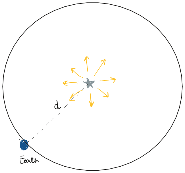
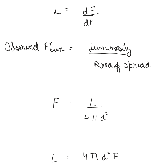
Where F is Flux or brightness and L is Luminosity and d is distance at which brightness or Flux is measured
Types
Luminosity and hence flux is observed and referred to in different ways and hence can be classified as following types
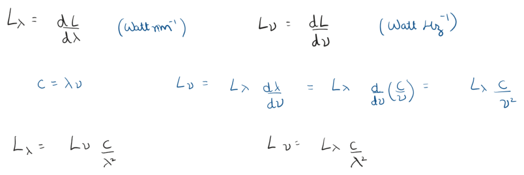
Spectral
Spectral Luminosity helps us see Luminosity distribution
Bolometric
Bolometric Luminosity shows brightness over the whole spectrum
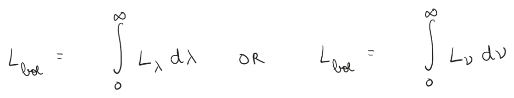
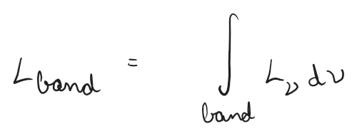
Band
Band Luminosity is often over a specific band (specific wavelength range)
Bands
There are different kind of photometric band systems used in astronomy:
Broadband
Broadband filters with a bandwidth greater than 30 nanometers, like:
Johnson-Morgan-Cousins (UBVRI) – (~365-820 nm) -> Ultraviolet – Near Infrared
SDSS (u′g′r′i′z′) – (~355-893 nm) -> Ultraviolet – Near Infrared
Gaia (G, BP, RP) – (~330-1050 nm) -> Ultraviolet – Near Infrared
2MASS (J, H, K_s) – (~1.11-1.32 micrometer) -> Near Infrared
WISE (W1–W4) – (3-22 micrometer) -> Mid Infrared
These are most commonly used as they help us know the colour, temperature, light variability etc. for most of the stars (which we’ll discuss in the later sections)
Intermediate
Intermediate which range from 10-30 nanometers like:
Stromgren (uvby) (350-547 nm)
These are used for specific purposes like capturing special characteristic features and metallicities to help classify stars.
Narrowband
Narrowband filters less than 10 nano meters like:
H_alpha
OIII (double ionized oxygen)
These are used to measure specific emission lines
Magnitude
Magnitude in context of stars is a logarithmic scale used to measure brightness of stars.
It is a backward scale (smaller magnitude = brighter object)
Apparent
Apparent magnitude is a measure of how bright the star appears to us.
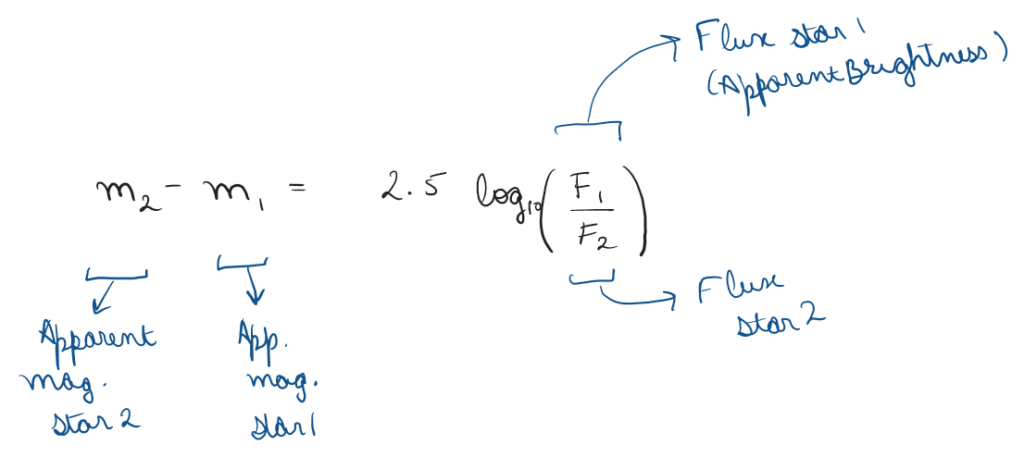
So a if a star is 1 magnitude less than the other, it would mean its ~2.512 times bright whereas if it was 5 magnitudes less it’d mean its 100x more bright!
e.g. Apparent magnitude of Saturn in 2025 ranged from ~ -0.6 – +1.4, apparent magnitude of our moon is ~ -12.7 (super bright!), for Polaris its close to ~ +2.0 and 3I Atlas (the popular comet of 2025) is currently at a magnitude of ~11 (here we just mentioned Visible range i.e. V band)
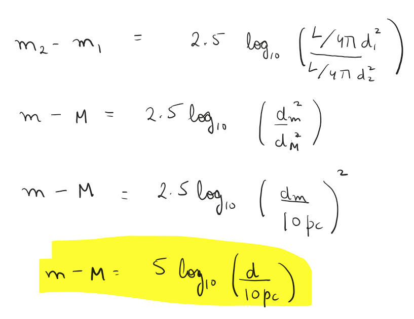
Absolute
Absolute magnitude is the magnitude of the star if it were at a standard distance of 10 parsecs.
e.g. Absolute magnitude of Saturn in 2025 ranged from ~ -9.5 to -10, absolute magnitude of our moon is ~ -0.2 to +0.2, for Polaris its close to ~ -3.6 to -3.7 and 3I Atlas (the popular comet of 2025) has an absolute magnitude of 12-13.7 (here we just mentioned Visible range i.e. V band)
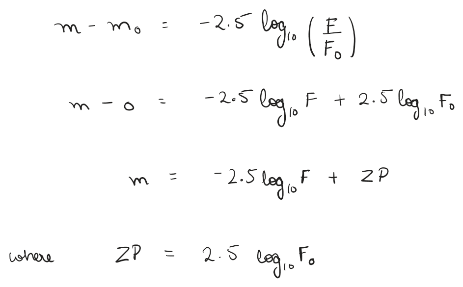
Zero Point
As you see above, magnitudes are defined on a relative scale (comparing relative brightness). Zero Point is the reference point, it is the brightness or flux that defines the magnitude 0.
Hence magnitude can be defined in comparison with zero point.
Magnitude Systems
There are several ways to look at magnitudes i.e. we can chose different reference spectrum and hence calibrate our data in different ways
AB
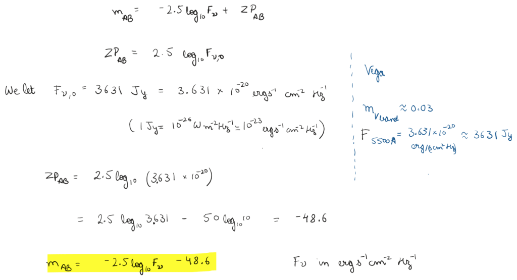
The AB system (tied to the ABsolute flux scale) is defined such that a flat spectrum in frequency (flux at a given frequency is constant) has same magnitude in all filters. This system is defined using flux density per unit frequency (f_nu) such that it has same magnitude in all filters. This system is popular in galaxy studies and cosmology.
For zero point we usually calibrate for the flat spectrum at 3631 Jansky (Jy) which actually corresponds to Vega in V band, it is mostly because this was well known historically.
ST
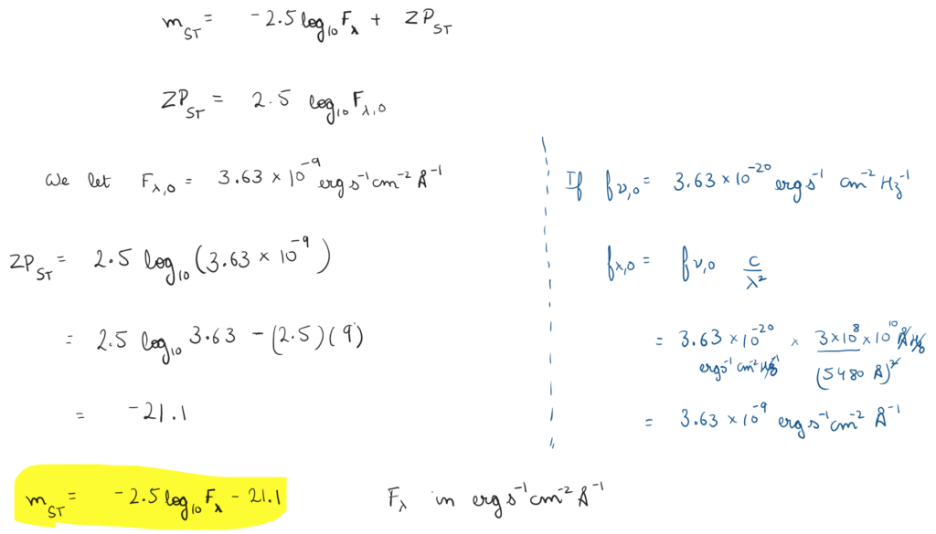
The ST (Space Telescope) system is very popular with Hubble Space Telescope studies and is defined such that a flat spectrum in wavelength (flux at a given wavelength is constant) has same magnitude in all filters. This system is defined using flux density per unit wavelength (f_lambda) such that it has same magnitude in all filters. This system is popular in spectroscopic studies.
For zero point we usually calibrate for the flat spectrum at 3.63e-9 ergs/s /cm / Angtrom corrosponding to the zero point frequency we took in AB system, this value gives zero point -21.1 but the wavelength considered is in Angstroms if the wavelength be in nanometers, the zero point would be -18.6
Vega
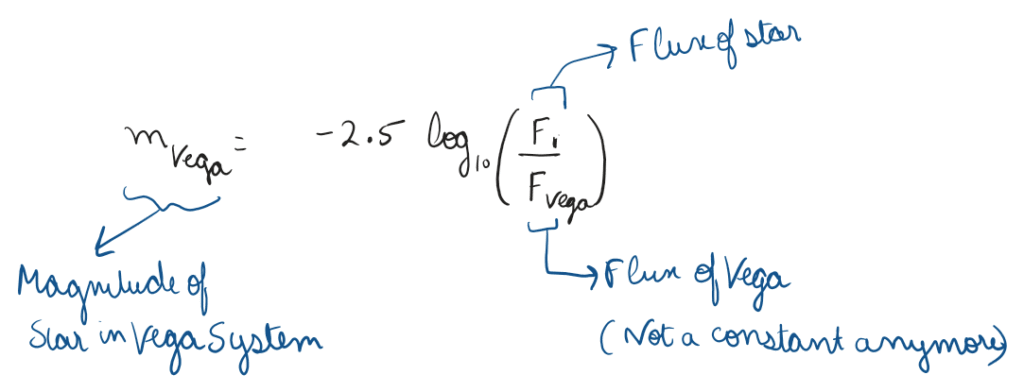
Vega magnitude system is one of the traditional systems used for stars, it is a relative system – in which star is compared to the star Vega and zero point is set such that apparent magnitude of Vega (m_Vega) = 0 in all bands
This system is filter dependent, i.e. it would be different for Johnson Cousins vs SDSS filters. Flux of Vega corrosponds to the Flux received from the star Vega in that band for that instrument.
We often need to switch magnitude systems and callibrate zero points espescially when consolidating different data sources or combining different attributes, this process is usually referred to flux callibration.
Extinction
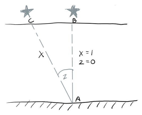
Extinction (k_lambda) and airmass (X) are the terms we account for in the apparent magnitude calculation that account for atmospheric interference
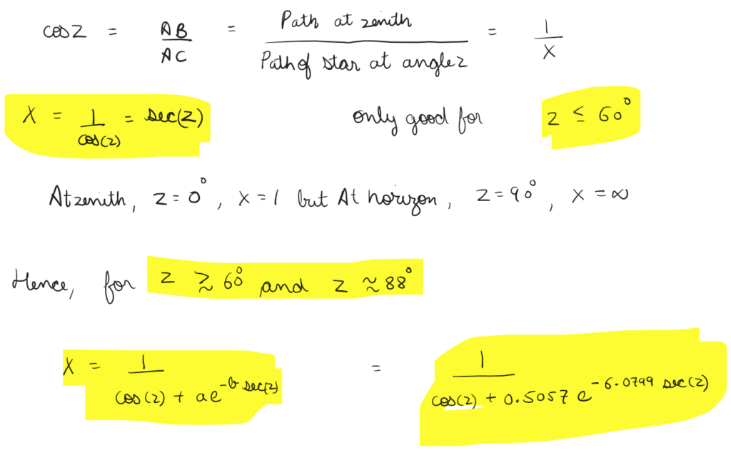
Airmass is defined as the amount of atmosphere light has to pass through to reach the instrument relative to the zenith.
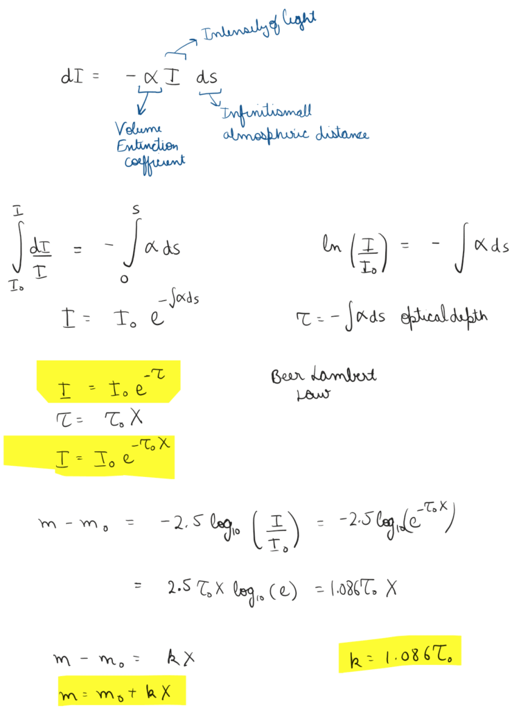
Extinction(k) is the reduction in intensity of light due to interactions with atmosphere.
References
Luminosity
Johnson-Morgan-Cousins
SDSS
Transformations between SDSS magnitudes and other systems
Historical View of the u’g’r’i’z’ Standard System
The ugriz Standard-Star System
Gaia
The design and performance of the Gaia photometric system
Gaia Early Data Release 3. Photometric content and validation
Gaia Data Release 1 , Gaia Data Release 3: External calibration of BP/RP low-resolution spectroscopic data
2MASS
Color Transformations for the 2MASS Second Incremental Data Release
The VISTA ZYJHKs photometric system: calibration from 2MASS
WISE
The Wide-field Infrared Survey Explorer (WISE): Mission Description and Initial On-orbit Performance
WISE Photometry for 400 Million SDSS Sources
Stromgen
A new catalogue of Strömgren-Crawford uvbyβ photometry
Interstellar reddening relations in the UBV, uvby, and Geneva systems
Flux Callibration
Zeropoints – Space Telescope Science Institute (STScI), Synthetic Photometry