Did you know NASA JPL has a service called Horizons which lets you look at mission statistics, here we try to predict the orbit and compare with Artemis I stats.
Orbital Mechanics is.. complicated, atleast to model with one equation, here we break the trajectory into multiple parts, first being the launch i.e. the Trans Lunar Injection (TLI) when the spacecraft is actually launched from the base with the rocket and the boosters, in this stage, there is a thrust generated by the engines, there is fuel depletion, different stages are let go gradually, the main forces are earth’s gravitation and atmospheric resistance and drag
Then there is 4 day trajectory to the moon, which is mostly coasting with little controlled thrust applied to control i.e. Thrust Control maneuvers (TCM)
In this project we focus on the Coasting part that is simulating the orbit under well a relatively stable and constrained environment.
Setup
We start with simple equations and simulate the trajectory, then compare to the actual data recorded and provided by JPL Horizons
We take some of our mission specific constants, like mass, area, engine thrust parameters from official website, and some of them from the engine manufacturer specification, as we said, to keep it simple we only consider the coasting phase right now and the engine used in that phase was ICPS – Interim Cryogenic Propulsion Stage which was developed by L3Harris, for planetary constants we use SPICE kernels, how they work is, we can put in the ID of specific planetary bodies and get their constant – this includes that of Earth (399), Moon (301), Sun and even of Artemis (-1023)! We get mission data (actual observed trajectory of Artemis – our ground truth) from JPL Horizons.
*JPL Horizons is in UTC but Spice is in Ephemeris Time
*Artemis I data in JPL is only during the TLI burn window
Here is how we get our observed Artemis Trajectory:
# Fetch Artemis I data during TLI burn
horizons_data_raw = fetch_horizons_vectors(
    target_id='-1023',
    center='@399',  # Earth-centered
    start_time='2022-11-16T08:47:00', # Post separation
    stop_time='2022-11-20T08:47:00',  # 4 days of cislunar coast
    step='10m'
) # => retuens time series of state vectors (position and velocities)
horizons_data = add_moon_distance_to_data(horizons_data_raw)
print(f"Retrieved {len(horizons_data['times_utc'])} data points")
print(f"Time span: {horizons_data['times_utc'][0]} to {horizons_data['times_utc'][-1]}")Retrieved 577 data points
Time span: A.D. 2022-Nov-16 08:47:00.0000 to A.D. 2022-Nov-20 08:47:00.0000
Now that we have, the observed data points , the first data point of the data we pulled being the closest index to flight ignition:
ECO index: 0 (t = A.D. 2022-Nov-16 08:47:00.0000)
Flight start index: 0 (t = A.D. 2022-Nov-16 08:47:00.0000)
Flight end index: 576 (t = A.D. 2022-Nov-20 08:47:00.0000)
we can check the velocity and position vectors it provides
Initial State (Earth-centered J2000):
  Position: [-3171.296, 9061.162, 5591.822] km
  Velocity: [-7.763256, 2.222213, 2.122515] km/s
  |r| = 11109.917 km (altitude: 4731.8 km)
  |v| = 8.349338 km/s (8349.3 m/s)
Total velocity change due to gravity during 4-day window: -8083.8 m/s
That is well above our Lower Earth Orbit (LEO) – and quite fast – between the velocity expected at LEO and the escape velocity (7.8-11.2km/s)
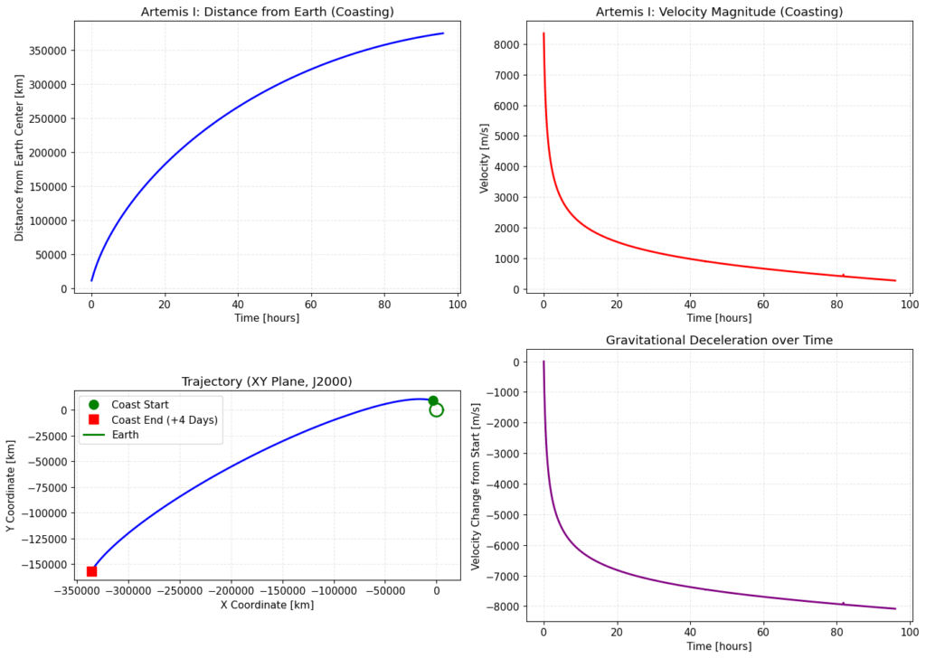
We see in our Plot 1 (top-left) – altitude steadily increasing as it moves from earth -> moon, the curve looks steep before but then flattens as it slows down
And in Plot 2 (top right) – after TLI burn, Orion is at ~8.3km/s, out of earth’s gravity, sun is probably pulling it back and its slowing down (the bump on 82hrs is another burn performed for trajectory correction)
Plot 3 (bottom left) – shows J2000 reference frame – top down view and Plot 4 (bottom right) shows cumulative velocity.
Now that we have the true observed data for the TLI window and mission constants, we try our basic physics on Artemis I.
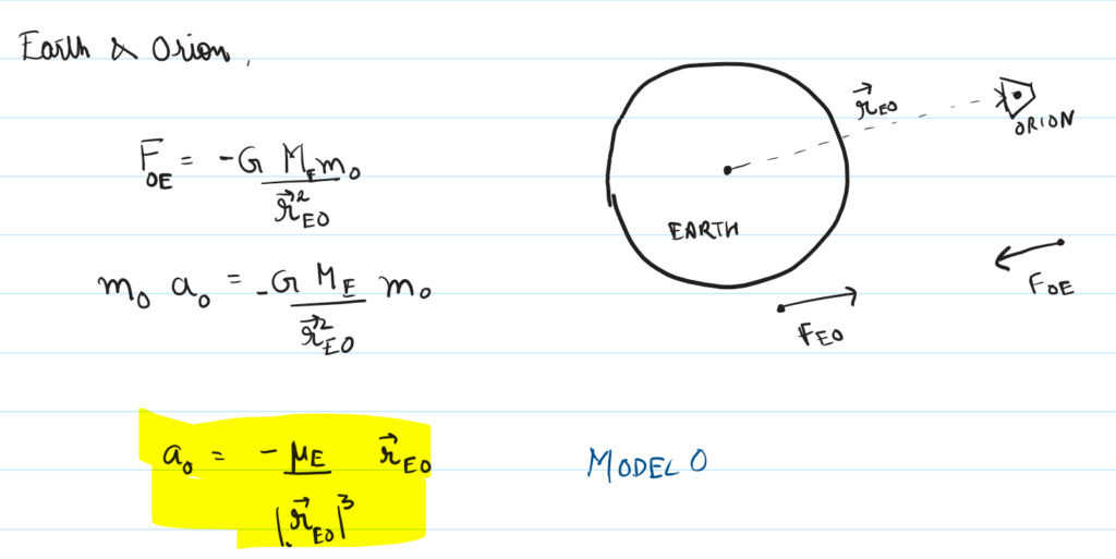
Two Body Integrator – Earth and Object
We start with a 2 body integrator – i.e. if gravity was the only force acting between the two bodies (our point mass of Orion and the Earth)
r: Position vector [km] (3,)
mu: Gravitational parameter [km^3/s^2]
def accel_two_body(r, mu=MU_EARTH):
    r_mag = np.linalg.norm(r)
    a = -mu * r / (r_mag ** 3) #[km/s^2] (3,)
return aFor now we’ll use traditional methods to solve this like the solve_ivp from scipy, we use Dormand Prince, the details you can see here
The equation we’re solving is:
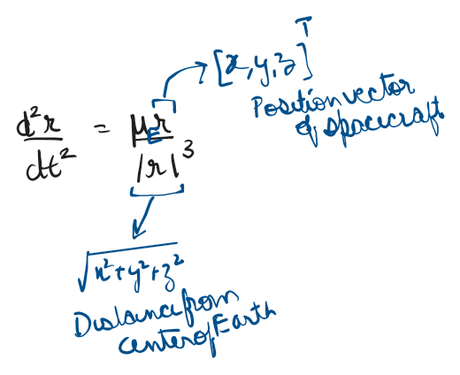
How it works with the data we fetched is:
This is essentially the equation and data we’re providing to our solver so it can predict the next position and velocity (helping us plot out the trajectory)
And here is the implementation of solve_ivp method:
def propagate_two_body(state0, t_span, t_eval=None, rtol=1e-10, atol=1e-12):
    def equations_of_motion(t, state):
        r = state[0:3]
        v = state[3:6]
        a = accel_two_body(r)
        return np.concatenate([v, a])

    sol = solve_ivp( # Solve Initial Value Problem
        equations_of_motion,
        t_span,
        state0,
        method='DOP853', #Runge-Kutta (Dormand-Prince 4th and 5th order)
        t_eval=t_eval,
        rtol=rtol,
        atol=atol,
        dense_output=True #spline
    )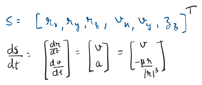
return solRemember our state vector s = [r_x, r_y, r_z, v_x, v_y, v_z]
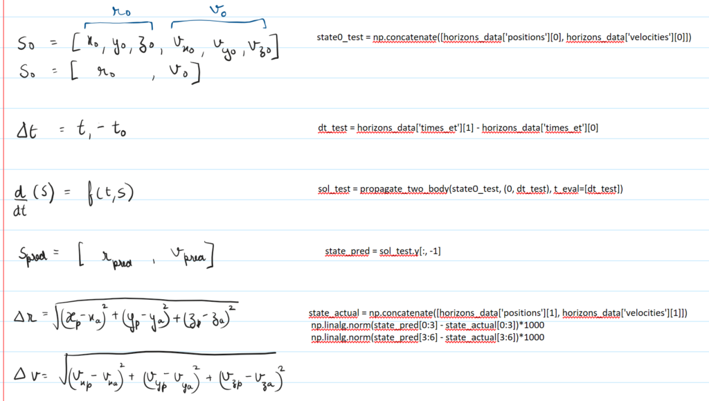
Start at position s0, assume only Earth’s gravity exists, integrate forward in time for dt_test seconds
s0: Test Coordinates (first position & velocity vector):
[-3.17129585e+03  9.06116222e+03  5.59182213e+03 -7.76325581e+00 2.22221349e+00  2.12251486e+00]
dt_test: delta t between first 2 data points: 600.0000001192093
Two-body baseline propagation (1-minute Post-TLI coast):
  Position error: 448.85 m
  Velocity error: 1.1021 m/s
so in about 60 seconds (1 minute) we missed our target by almost half a km! if we use our Model 0 equation that just accounts for earth’s gravity treating the problem like a 2 body problem.
When we run this over 4 days (i.e.e our entire set of data points) for the whole coast duration, we end up being off by ~9747.82 km
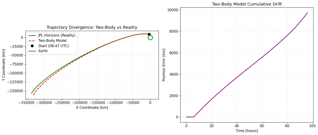
Where the plot on left shows the top down 2D view of different trajectories, showing divergence of our simplistic 2 body trajectory calculated (red dashed line – made of s_pred) with the one executed(green – horizon’s data)
and plot on the right, shows positional error over time, at 96hrs (4 days) it is ~10,000 km off
J2 Oblateness – Earth
The first and most significant gravitational perturbation comes from the shape of the Earth itself, because the Earth spins on its axis, centrifugal force flattens the poles and flings material outward at the equator, creating an equatorial bulge.
This uses Laplacian in spherical coordinates which you can find here and spherical harmonics, more about that later.
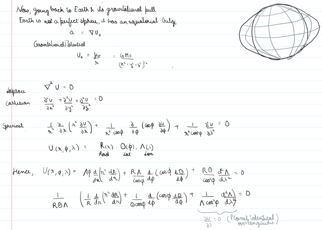
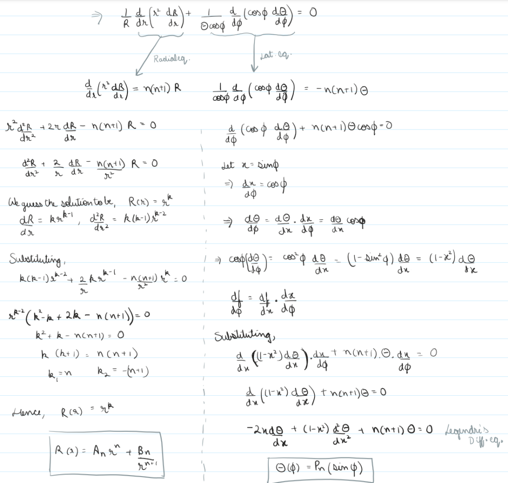
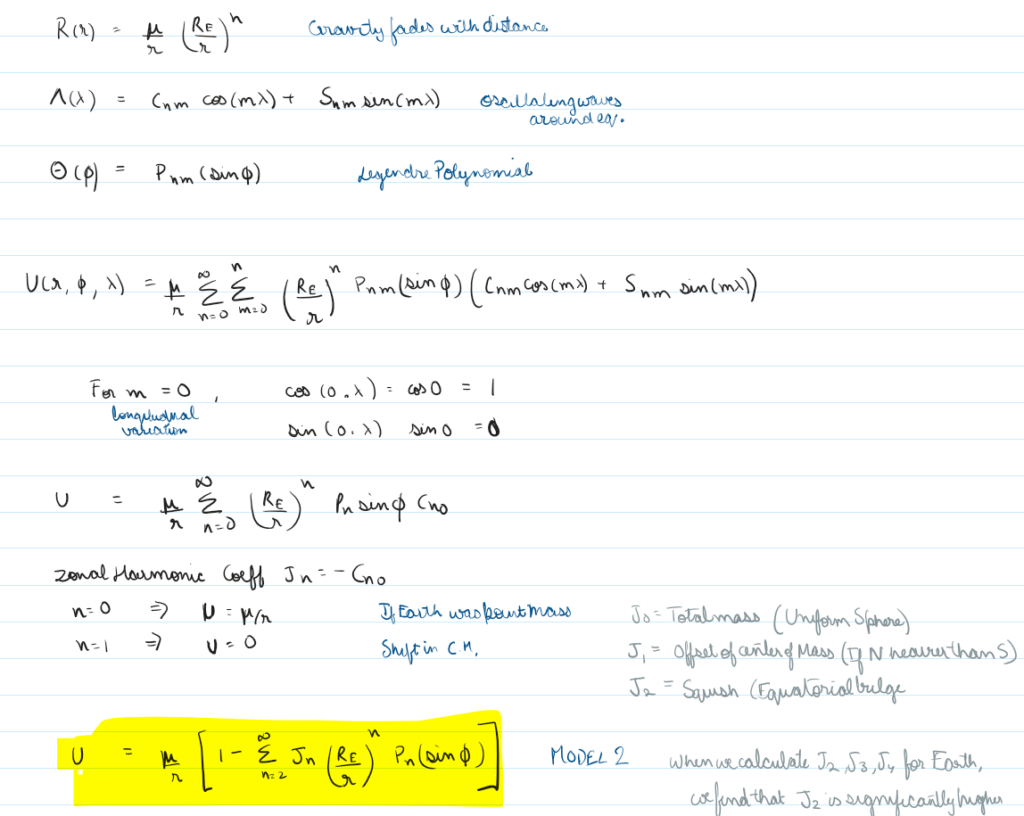
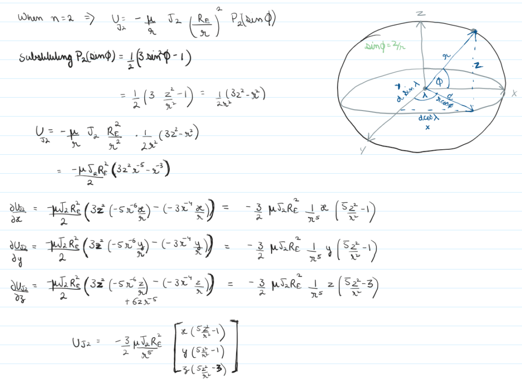
Hence our equation accounting for modified gravitation potential becomes:
In python it’d look like:
def accel_j2(r, mu=MU_EARTH, j2=J2_EARTH, r_eq=R_EARTH):
    x, y, z = r
    # z=0, spacecraft directly above equator, if z is really large, its probably over the poles
    r_mag = np.linalg.norm(r)
    r2 = r_mag ** 2
    r5 = r_mag ** 5

    z2_r2 = (z ** 2) / r2

    # coeff = -1.5 * j2 * mu * (r_eq ** 2) / r5
    coeff = 1.5 * j2 * mu * (r_eq ** 2) / r5

    a_x = coeff * x * (5 * z2_r2 - 1)
    a_y = coeff * y * (5 * z2_r2 - 1)
    a_z = coeff * z * (5 * z2_r2 - 3)

    return np.array([a_x, a_y, a_z])

def accel_two_body_j2(r):
    return accel_two_body(r) + accel_j2(r)
def propagate_earth_j2(state0, t_span, t_eval, gravity_func, rtol=1e-10, atol=1e-12):
def equations_of_motion(t, state):
r = state[0:3]
v = state[3:6]
a = gravity_func(r)
return np.concatenate([v, a])
return solve_ivp(equations_of_motion, t_span, state0, method='DOP853',
t_eval=t_eval, rtol=rtol, atol=atol)We use the same solver DOP853 and test for the initial point again and get:
Acceleration comparison at initial position:
  Two-body: 3.229358 m/s² (3229.358 mm/s²)
  J2:       1.559640 mm/s²
  J2/2body ratio: 0.0483%
The standard, point mass gravity of the Earth is pulling backward on the spacecraft at 3.23m/s^2. This is the primary engine of orbital mechanics, keeping the capsule trapped in a curved trajectory rather than flying off into a straight line into deep space.
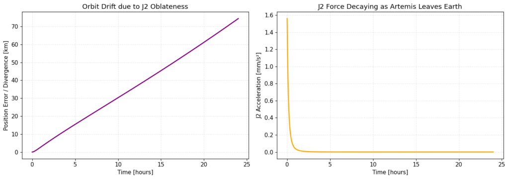
The extra gravitational pull caused by the Earth’s fat equatorial bulge (J2) is applying an extra acceleration of 1.56 mm/s^2 roughly 0.05% of primary force (discarding the deviation or Earth’s shape from a perfect sphere) i.e. if we keep everything else identical but ignore the planet’s shape, the model will drift by exactly 74.38 km after one day
Now when we run for the whole trajectory (i.e. the data points observed), and compare Euclidean vector distance between our previous model and this new model that accounts for earth’s oblateness and plot it over 24 hours (left) and we see an error of 74.8 km
While our position divergence increases with time, our plot of the J2 force magnitude plummets off a cliff, dropping to near zero within the first 5 hours. Because J2 decays at a brutal spatial power law of 1/r^4, the shape of the Earth matters immensely while the spacecraft is close to home, but it quickly becomes a mathematical ghost as Artemis escapes into deep space on its way to the Moon
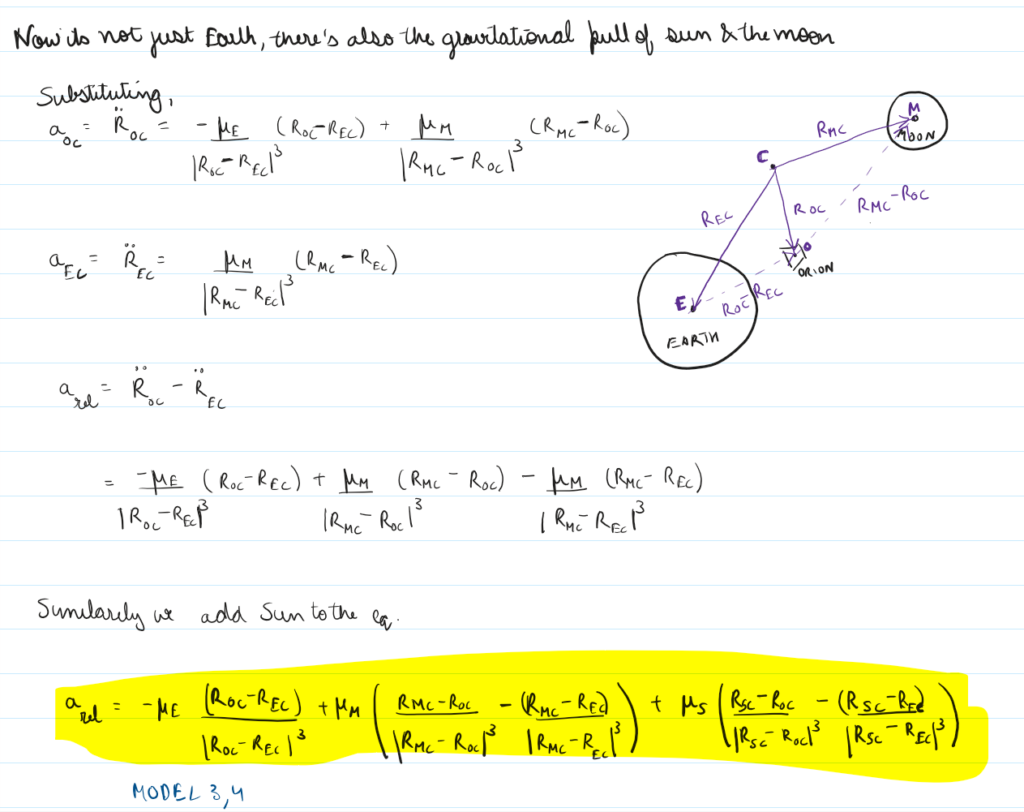
Third Body Perturbations – Sun and Moon
As the spacecraft leaves earth’s orbit, we’re forced to account for the gravitational effects of other bodies i.e. the moon and the sun, but because our entire tracking coordinate system is anchored directly to the center of the Earth, we cannot just add a standard Newtonian gravity vector, so, we use relative third body acceleration.
Now putting this in code:
def accel_third_body(r_sc, r_body, mu_body):
    # Direct Term: Acceleration of Spacecraft toward Third Body
    r_body_to_sc = r_sc - r_body
    a_direct = -mu_body * (r_body_to_sc / np.linalg.norm(r_body_to_sc)**3)
    # Indirect Term: Acceleration of Earth toward Third Body
    a_indirect = mu_body * (r_body / np.linalg.norm(r_body)**3)
    # Relative Acceleration: Spacecraft minus Earth
    return a_direct - a_indirect

def accel_moon(r_sc, et):
    r_moon = get_body_position_spice(301, 399, et)  # Moon wrt Earth
    return accel_third_body(r_sc, r_moon, MU_MOON)

def accel_sun(r_sc, et):
    r_sun = get_body_position_spice(10, 399, et)  # Sun wrt Earth
    return accel_third_body(r_sc, r_sun, MU_SUN)
def propagate_nbody(state0, t_span, t_eval, et_start):
def equations_of_motion(t, state):
r = state[0:3]
v = state[3:6]
current_et = et_start + t #SPICE needs the exact current time
# Calculate all forces
a_earth = accel_two_body_j2(r) # Earth + Bulge
a_m = accel_moon(r, current_et) # Moon
a_s = accel_sun(r, current_et) # Sun
return np.concatenate([v, a_earth + a_m + a_s])
return solve_ivp(equations_of_motion, t_span, state0, method='DOP853',
t_eval=t_eval, rtol=1e-10, atol=1e-12)Running the test for first point:
Third-body accelerations at TLI ignition:
  Moon: 1.506 nm/s² (direction: [-0.943, 0.282, 0.175])
  Sun:  0.653 nm/s²
  Moon/J2 ratio: 0.0966%

Moon distance from Earth: 402232 km
At the moment the rocket engines ignite, the gravitational pull of the Moon acts as a literal whisper, registering at just 1.506 nm/s^2 and the Sun is even weaker, pulling at 0.653 nm/s^2, and at the start of the lunar voyage, the subtle asymmetry of Earth’s equatorial bulge (J2) is over 1000 times more powerful than the direct gravitational pull of the Moon
Now running for four days:
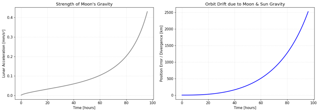
The left plot tracks the absolute strength of the Moon’s gravity acting on Orion as the hours tick by. For the first 40 hours of the trip, the line remains low and flat. Earth’s heavy mass is the dominant factor, but as the capsule puts more distance between itself and Earth, the curve suddenly reaches an inflection point and skyrockets, ramping all the way up to 14 mm/s^2 by hour 96. Lunar Sphere of Influence (SOI). The deep space whisper we detected at ignition has officially scaled into the dominant tractor beam that will determine whether the capsule circles the Moon or gets flung hopelessly out into deep solar space.
The right plot illustrates the compounding tracking penalty if you choose to pretend the Moon and Sun do not exist. For the first two days, the error barely registers. But as the capsule climbs higher into the cislunar landscape, the omission of third-body forces catches up with the model with a vengeance. By the end of the 4-day window, our Earth only prediction drifts off course by a massive 2,527.79 kilometers.
Radius of the Moon is roughly 1,737 km, Artemis I was targeting a highly precise flyby altitude of just 130 km above the lunar surface, if a mission planner used a simple Earth-only Two-Body model and ignored the Moon and Sun, their math would put them 2,500 km off target.
Solar Radiation Pressure
Photons streaming from the Sun carry momentum. When they smash into the reflective surfaces and solar panels of the Orion capsule, they transfer that momentum, acting like a continuous, ultra-faint cosmic wind pushing the spacecraft directly away from the Sun.
However, before we can calculate this photon push, we have to solve another problem: The Eclipse. If the Earth blocks the line of sight between the spacecraft and the Sun, the spacecraft plunges into darkness, and the solar pressure drops instantly to zero.
To track this, we write a vector based cylindrical shadow function:
def is_in_shadow(r_sc, r_sun, r_body=R_EARTH):
    # Unit vector from Earth to Sun
    r_sun_mag = np.linalg.norm(r_sun)
    sun_hat = r_sun / r_sun_mag
    # Project spacecraft position onto Sun direction
    proj = np.dot(r_sc, sun_hat)
    # If spacecraft is on Sun side, not in shadow
    if proj > 0:
        return 1.0
    # Perpendicular distance from shadow axis
    perp = r_sc - proj * sun_hat
    perp_dist = np.linalg.norm(perp)
    # Simple cylindrical shadow
    if perp_dist < r_body:
        return 0.0
return 1.0If our capsule passes the shadow test, we can calculate the Solar Radiation Pressure acceleration vector using the radiation pressure coefficient. At a standard distance of 1 Astronomical Unit (1 AU) from the Sun, the solar constant delivers a radiation pressure of roughly 4.56e-6 N/m². Our script scales this base pressure inversely with the square of our dynamic distance from the Sun
Implementing it:
def accel_srp(r_sc, mass, et, cr=CR_SRP, area=ORION_AREA):
    # Sun position wrt Earth
    r_sun_earth = get_body_position_spice(10, 399, et)

    # Spacecraft to Sun vector
    r_sc_to_sun = r_sun_earth - r_sc
    r_sc_sun_mag = np.linalg.norm(r_sc_to_sun)
    sun_hat = r_sc_to_sun / r_sc_sun_mag

    # Check shadow
    shadow = is_in_shadow(r_sc, r_sun_earth)
    if shadow == 0:
        return np.zeros(3)

    # SRP pressure at 1 AU: P = Phi/c
    # Phi = 1367 W/m^2, c = 299792458 m/s
    # P_1AU = 1367 / 299792458 = 4.56e-6 N/m^2
    P_1AU = SOLAR_FLUX / (C_LIGHT * 1000)  # N/m^2 (c in m/s)

    # Scale by distance
    r_sc_sun_au = r_sc_sun_mag / AU_KM
    P = P_1AU / (r_sc_sun_au ** 2)

    # Acceleration: a = Cr * P * A / m
    # Units: a [m/s^2] = Cr * P [N/m^2] * A [m^2] / m [kg]
    a_mag = cr * P * area / mass  # m/s^2
    a_mag_km = a_mag / 1000.0  # km/s^2

    # Direction: away from Sun
    # SRP acceleration [km/s^2]
return -a_mag_km * sun_hat * shadowUsing the same solver:
def propagate_srp(state0, t_span, t_eval, et_start, mass, include_srp=True):
    def equations_of_motion(t, state):
        r = state[0:3]
        v = state[3:6]
        current_et = et_start + t

        r_sun = get_body_position_spice(10, 399, current_et)
        r_moon = get_body_position_spice(301, 399, current_et)

        a_earth = accel_two_body_j2(r)
        a_moon = accel_third_body(r, r_moon, MU_MOON)
        a_sun = accel_third_body(r, r_sun, MU_SUN)
        a_srp_force = accel_srp(r, mass, current_et) if include_srp else np.zeros(3)

        # The sum of all forces acting on the spacecraft
        return np.concatenate([v, a_earth + a_moon + a_sun + a_srp_force])

    return solve_ivp(equations_of_motion, t_span, state0, method='DOP853',
t_eval=t_eval, rtol=1e-10, atol=1e-12)Running it on the first point to test:
SRP acceleration at TLI: 6.596 pm/s²
SRP/Moon ratio: 0.4380%
Shadow factor: 1.0
At launch, the photon pressure acting on Orion registers at a mind bogglingly tiny 6.596 picometers per second squared. A picometer is one trillionth of a meter. This force is so incredibly weak that it makes the Moon’s gravity look like a powerhouse by comparison, accounting for a mere 0.4380% of the lunar pull.
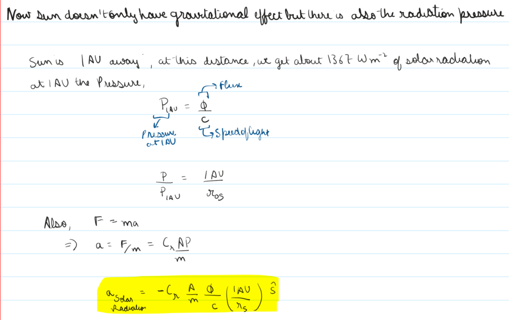
When we run it for the whole trajectory (we actually run twice, with SRP and without to compare the effect):
Our first plot (left) shows that as Artemis sails toward the Moon, the absolute magnitude of the solar pressure acceleration stays relatively stable, hovering right around the 0.0057 nm/s² range. Because a 4 day trip to the Moon barely changes our total distance relative to the massive 150-million-kilometer orbit of the Sun, the solar wind acts as a completely steady, relentless push.
Our second plot (right) tracks the absolute spatial divergence between our gravity only model and our photon-powered model, over 4 days this tiny affect actually moves the spacecraft ~0.45 km
J2 Oblateness – Moon
The Moon itself isn’t a perfect sphere either. The Moon has its own equatorial bulge, quantified by its own J2 value. We can’t really use our previous J2 approach that we applied to Earth because the J2000 coordinate system is anchored directly to Earth’s center of mass, and its vertical z-axis points directly out of Earth’s North Pole. Because Earth’s rotational axis stays fixed relative to this grid, our coordinate framework lines up with the shape of the planet. But the Moon is orbiting, drifting, and tilted relative to Earth. The Moon’s personal north pole is pointing in a completely different direction than Earth’s.
To figure out how the Moon’s shape is pulling on the spacecraft, we must step out of the static, inertial universe and jump into a rotating frame:
- Step 1: We calculate the relative distance vector from the Moon to the spacecraft in the standard inertial frame (
J2000) - Step 2: We query SPICE to get a dynamic rotation transformation matrix (
spice.pxform) that matches the exact microsecond of our flight time. We use this matrix to rotate our position vector into the Moon’s body-fixed, rotating frame (IAU_MOON). In this frame, the z-axis points squarely out of the Moon’s true rotation axis. - Step 3: Now that our coordinates are properly aligned with the Moon’s geometry, we pass them through our standard
accel_j2function using lunar mass and lunar radius - Step 4: This gives us an acceleration force vector mapped in the Moon’s frame. To feed this force back into our main tracker, we use a reverse rotation matrix to shift that acceleration vector straight back out into the
J2000inertial system
def accel_j2_moon(r_sc, et):
    r_moon = get_body_position_spice(301, 399, et)
    # r_sc_moon = r_sc - r_moon
    # return accel_j2(r_sc_moon, mu=MU_MOON, j2=J2_MOON, r_eq=R_MOON)
    r_sc_moon_j2000 = r_sc - r_moon
    # J2 must be computed in the body-fixed frame, not inertial J2000.
    rot_j2000_to_moon = spice.pxform('J2000', 'IAU_MOON', et)
    rot_moon_to_j2000 = spice.pxform('IAU_MOON', 'J2000', et)
    r_sc_moon_fixed = rot_j2000_to_moon @ r_sc_moon_j2000
    a_j2_fixed = accel_j2(r_sc_moon_fixed, mu=MU_MOON, j2=J2_MOON, r_eq=R_MOON)
    return rot_moon_to_j2000 @ a_j2_fixed
def propagate_moon_j2(state0, t_span, t_eval, et_start, mass):
def eom(t, state):
r, v = state[0:3], state[3:6]
et = et_start + t
a = (accel_two_body_j2(r) + accel_moon(r, et) + accel_sun(r, et) +
accel_srp(r, mass, et) + accel_j2_moon(r, et))
return np.concatenate([v, a])
return solve_ivp(eom, t_span, state0, method='DOP853', t_eval=t_eval, rtol=1e-10, atol=1e-12)
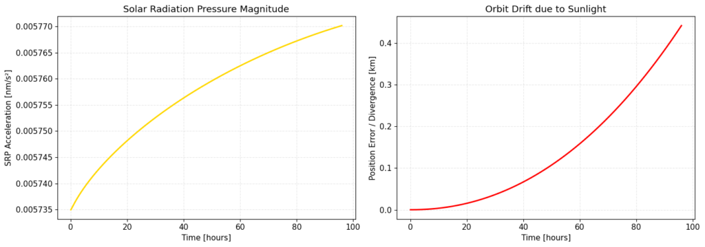
The left plot tracks the raw acceleration magnitude exerted on Orion by the Moon’s equatorial bulge (J2) over the final 24 hours leading up to its close approach, as the clock ticks past hour 20, the spacecraft gets close to its target. In the final two hours, the force curves upward like a vertical cliff face.
The spatial proximity factor has officially taken complete control of the simulation. Because the spacecraft is reaching its absolute closest point to the lunar surface (perilune), the non-linear 1/r^5 power law of the J2 multiplier explodes, utterly overwhelming the latitude variations and creating a massive gravitational spike
The right plot tracks the spatial divergence (div_super_km) between the model with and without Lunar J2. The y-axis scale is incredibly tiny, topping out at around 0.000035 km (3.5 cm). You noted that at the end of the day, the final displacement is only 3.2 centimeters.
The unique, wavy shape of that specific plot is caused by the geometric focusing pocket of the Moon’s central gravity well pulling the two paths together before they snap apart.
Now you’ll ask why do we see that wavy thing on the right plot and not on the left, its because left plot is snapshot of instant of time, doesn’t care about trajectory history, right plot measures the accumulated path distance error over time. This distance gap is a dynamic entity. It is being pulled on by two different forces simultaneously: the lumpy Lunar J2 perturbation, and the massive, baseline point mass gravity of the Moon.
We sliced a 4 day simulation at the 72 hour mark to capture the final 24 hours. Because our previous simulation already having minor rounding drifts and solar radiation pressure shifts, the initial state vector already carried a small baseline velocity and position mismatch relative to the Moon
Hour 0-12 – As the simulation kicks off, the initial baseline velocity mismatch causes the two virtual spacecraft to drift apart, climbing up to 1.8 centimeters. At this distance from the Moon (hundreds of thousands of kilometers out), the local Lunar J2 force (Left Plot) is weak, so it isn’t contributing much yet. This initial hill is just the standard kinetic drift from initial conditions
Hour 12-20- Because the Moon’s core central gravity pulls everything directly toward its center of mass, it acts as a geometric lens. It physically pinches the two independent trajectories closer together. On right-hand plot, this gravitational focusing causes the distance error to shrink, dropping from 1.8 cm down to a local trough of 1.3 cm
But right at Hour 22, the spacecraft slams directly into the Lunar J2 acceleration wall seen on the left plot. At a close approach of just a few hundred kilometers, the Moon’s squashed, asymmetrical shape exerts a sudden, violent torque on the velocity vectors. Because the two spacecraft are at slightly different latitudes, this asymmetric bulge pulls on one capsule harder than the other. This gravitational shear completely overpowers the central focusing funnel, violently tearing the two paths apart in a sharp terminal hook that shoots up to 3.2 centimeters right at perilune
And well after all this dissection, the fact is, the impact of moon’s oblateness as you see in centimeters, so we’re gonna ignore this right now.
Conclusion
What we have so far is:
# Setup exact timestamps and ground truth data
t_eval_exact = horizons_data['times_et'] - t_start_et
h_pos = horizons_data['positions']
h_vel = horizons_data['velocities']
time_hours = t_eval_exact / 3600.0

# Extract Moon distance
moon_dist = horizons_data.get('moon_distances')

# Propagate all intermediate models at the exact Horizons timestamps
sol_2body_exact = propagate_two_body(state0_test, (0, dt_test), t_eval=[dt_test])
sol_j2_exact = propagate_earth_j2(state0_coast, (0, t_eval_exact[-1]), t_eval_exact, accel_two_body_j2)
sol_nbody_exact = propagate_nbody(state0_coast, (0, t_eval_exact[-1]), t_eval_exact, t_start_et)
sol_ult_exact = propagate_srp(state0_coast, (0, t_eval_exact[-1]), t_eval_exact, t_start_et, COASTING_MASS, include_srp=True)

# Calculate position errors against Horizons for each model
error_2body = np.linalg.norm(sol_2body_exact.y[0:3, :].T - h_pos, axis=1)
error_j2    = np.linalg.norm(sol_j2_exact.y[0:3, :].T - h_pos, axis=1)
error_nbody = np.linalg.norm(sol_nbody_exact.y[0:3, :].T - h_pos, axis=1)
error_ult   = np.linalg.norm(sol_ult_exact.y[0:3, :].T - h_pos, axis=1)

velmag_ultimate = np.linalg.norm(sol_ult_exact.y[3:6, :], axis=0)
velmag_horizons = np.linalg.norm(h_vel, axis=1)And we get:
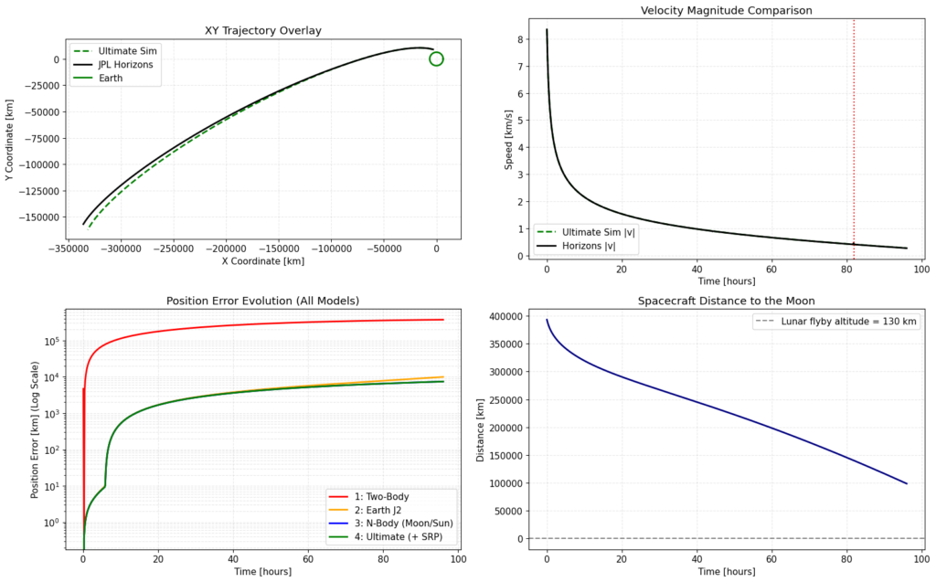
Plot Top-Left
In a 2D XY trajectory overlay, our green dashed line (Ultimate Sim) and the black line (JPL Horizons) map out an identical path. They appear perfectly matched for the most part and deviate slightly. This kinda also demonstrates a dangerous visual trap in deep space mapping (or well anything on such astronomical scales): planetary scales mask massive operational drifts. Because cislunar space spans hundreds of thousands of kilometers, a tracking mismatch of several thousand kilometers looks like a minor pixel variation. We have to dive into the mathematical residuals to find the true story. (or plot these differences on a logarithmic scale)
Plot Top-Right
This tracks our predicted velocity magnitude against reality. Both tracks capture the expected kinetic deceleration as Orion climbs out of Earth’s heavy gravity well, dropping from 8.3 km/s down toward a 1-2km/s coast.
However, notice the sudden separation around the 82-hour mark (highlighted by the red vertical dotted line). The real-world tracking telemetry registers a distinct speed profile shift that our passive simulator misses entirely. Because a natural force like gravity does not suddenly switch gears like an automatic transmission, this is our first clear sign of a propulsive system actively firing. (TCM maneuver)
Plot Bottom-Left
This uses a logarithmic scale to show the cumulative position error over time for all four configurations. It clearly maps the hierarchy of cislunar forces:
- Model 1: Pure Two-Body (Red Line): Explodes off the charts almost instantly, crossing the 1,000 km error mark within the first 12 hours. It finishes completely broken, nearly 10,000 km off target.
- Model 2: Earth J2 (Orange Line): Marginally safer during the first few hours, but follows the exact same catastrophic curve once the capsule leaves low Earth altitudes.
- Model 3: N-Body Gravity (Blue Line): The moment the moving gravitational wells of the Moon and Sun are introduced via SPICE, the error profile drops by orders of magnitude. The error line flattens out, illustrating how n body gravity stabilizes our system.
- Model 4: Ultimate with SRP (Green Line): Adding the faint push of solar radiation pressure strips away even more residual drift, yielding the lowest baseline error profile of any model.
Despite matching reality with exceptional precision for the first half of the journey, our ultimate model hits a hard wall in the final leg of the transit, concluding with a final tracking error of 7,426.285 km.
Plot Bottom-Right
Our final panel tracks our straight-line distance to our target destination: the Moon. It maps our steady descent down into the lunar realm, highlighting a gray baseline of 130 km, NASA’s targeted close approach flyby altitude.
Because our passive simulation missed by over 7,400 km, our virtual version of Orion completely overshot this insertion window, sailing right past the lunar sphere into deep solar space.
Why did our meticulously designed simulator miss by thousands of kilometers?
Our ultimate model represents a universe where Artemis I is a totally passive, drifting rock. We don’t account for fuel consumption (change in mass), TCM (active steering) etc.
To better encapsulate the known physics, we need to do the above and in addition, use higher order harmonics for earth, earth’s tidal fluctuations can also affect earth’s gravity (the bulge can vary a lot in mass and radius), the J2 we derived isn’t static.
Even moon has weird mass concentrations causing lumpy gravity which we did not consider here, NASA apparently uses another equation for lunar gravity derived from their past mission observations
And well Newtonian gravity is an approximation – we need to use GR corrections for our massive spinning Earth
Even the SRP interacts causing secondary light and heat on the spacecraft, earth and the moon (earthshine and moonshine) although those effects are usually very small in nanometer – picometer scale – but they’re variable as well.
In our equations we also didn’t account for our atmospheric drag, even in LEO the atmospheric drag is significant – however it is 0 in the cis lunar coast, but significant at launch and re entry.
Here in this post we tried to use our physics intuition and used numerical solvers for the differential equations we framed to describe the trajectory, then we compared it with the observed data of the mission.
What we built in Python is a Forward Propagator. We gave it a starting point, hit “go,” and watched where the physics took it. But NASA doesn’t just guess and wait, they use a continuous, closed loop feedback system that mathematically stitches the simulation to real world data
They don’t have a database of positions perfectly handed to them. They have to measure the spacecraft from Earth using the Deep Space Network, once they have the noisy radio data, they feed it into their enterprise software (like MONTE). But instead of just plotting it, they run an Extended Kalman Filter (EKF) or a Batch Least Squares estimator:
This is where the magic happens:
- The software runs the Cowell’s Formulation physics simulation forward by one step.
- It predicts what the DSN radio signal should look like based on that physics model.
- It compares the prediction to the actual noisy radio data received from the spacecraft to generate a residual (like our error plots)
- Using complex matrix calculus (Jacobians), the filter calculates exactly how much it needs to tweak the spacecraft’s velocity, position, and assumed forces to make the error drop to zero
In the next post we will see how PINNs fare with this problem. Stay Tuned
Leave a Reply