In our previous posts, we reached the limits of both the classical and computational worlds. Traditional numerical solvers, like Finite Element Methods (FEM) or LSODA are rigorous, but they are computationally crippling. Simulating the hypersonic fluid dynamics of a re-entering spacecraft or forecasting global spatiotemporal weather anomalies can take supercomputers days or weeks.

We need the simulations to be faster.

For the last decade, the tech industry’s answer to speed has been Machine Learning. We train massive Deep Neural Networks to look at past data and instantly predict the future – they act almost as Universal Function Approximators. But when applied to deep physical sciences, standard Artificial Intelligence has a fatal flaw: it is completely physically illiterate.

If you train a standard neural network on atmospheric telemetry, it kind of acts like a highly advanced curve fitter. It might predict a weather front or an orbital trajectory that explicitly violates the conservation of mass, energy, or momentum, simply because it doesn’t “know” those laws exist, it could predict that mass is being spontaneously created out of nowhere, or that water is flowing uphill, simply because it found a statistical shortcut.

To model the future of the cosmos, we cannot just rely on pure data, nor can we rely on pure computation. We have to merge the two.

And that is the basis of PINNs – Physics Informed Neural Networks

Instead of forcing a computer to blindly calculate a physical grid, or blindly memorize a dataset, a PINN is a neural network that has the laws of physics mathematically baked directly into its brain.

The Idea

In traditional Machine Learning, when a model overfits sparse data, we use regularization (like L1 or L2 penalties) to artificially restrict the network’s weights and keep the predictions smooth.

Instead of arbitrarily penalizing large weights like that, a PINN uses the actual differential equations of the physical system (the ODEs or PDEs) as the ultimate regularization term. By encoding the laws of physics directly into the network, we inject a massive, undeniable prior. We forcefully restrict the space of admissible solutions. The network is no longer allowed to guess anything that violates the conservation of mass, energy, or momentum

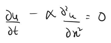
Let’s take an example of the heat equation:

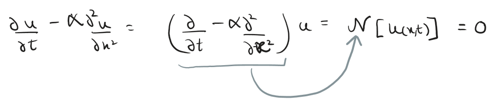
Abstracting the operator and simplifying notations for ML math:

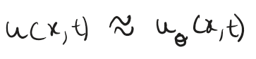
Now with Neural networks, instead of finding exact u(x,t) we approximate it using learned weights and biases of the network (theta)

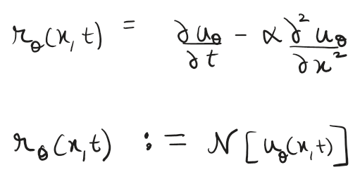
Now we define a residual function for the network which measures how much our network’s output violates the PDE

The purpose of a Neural Network model is to find specific network parameters (weights and biases – theta) that minimize loss (L)

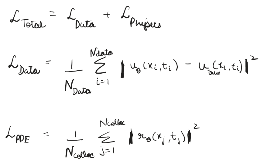
Here we define our loss as a combination of data loss and physics loss (Which is driven by our residual function which is essentially modelled as a PDE) – hence directly baking in the physics into a neural network.

Working

We will walk through how a PINN works using a general case

Point Generation

In traditional numerical solvers (like FDM or FEM), discretizing the universe is an agonizing process. You must build a rigid, perfectly interconnected grid or mesh. Generating a mesh that seamlessly wraps around without creating mathematical singularities can sometimes take an engineer days and in high dimensional physics, the number of grid points required explodes exponentially, a curse of dimensionality.

Because Physics Informed Neural Networks use Automatic Differentiation, they don’t care about grids. They evaluate spatial and temporal derivatives continuously. However, to compute the Physics Loss, we still have to tell the network where to check the physics.

We do this by generating Collocation Points, empty coordinates in space and time where we enforce the differential equation

Boundary / Initial Points which are derived from BVP and IVP

Collocation Points which are points generated by statistical sampling of random points inside the domain

If we just scatter them completely randomly (Standard Monte Carlo), we risk leaving massive blind spots in our physical domain where the network can essentially cheat and ignore the physics. One of the most popular algorithms to do this statistical sampling is Latin Hypercube Sampling (LHS) which ensures our points are maximally spread out with equal probability bin.

There are also some techniques of Adaptive Sampling. As the neural network trains, we constantly monitor the physical residual (f) at all of our collocation points. If the network calculates a massive physics loss in a specific sub-region (indicating it is struggling to understand the math there), the algorithm dynamically generates thousands of new collocation points specifically clustered around that high-error zone.

All these values values for collocation points are stored as tensors

Forward Pass

We feed the neural network raw continuous coordinates: space (x) and time (t). The network acts as our universal approximator and spits out a predicted physical state, u_theta(x,t)

The neural network is no longer trying to find a correlation in a dataset. The neural network has literally become the mathematical function. It is a parameterized surrogate for the true, undiscovered analytical equation

In case of a simple multilayer perceptron (fully connected layers)

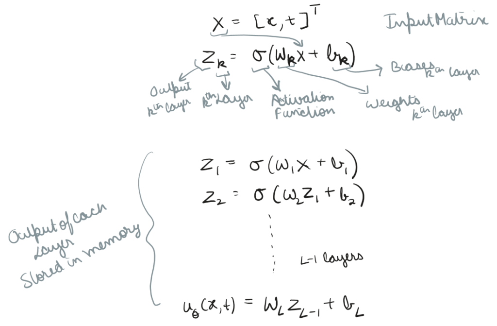
The output of each layer is stored and parallel matrix dot product computed simultaneously across all points.

Auto Differentiation

To calculate the first and second derivatives required in our residual function, we use backward chain rule on the composite function

For instance, if the network had only one hidden layer

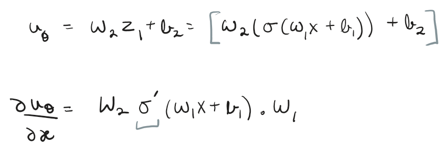
Because PINNs use exact derivatives of activation functions, we tend to use smooth functions like tanh

In this step we are traversing back the computation graph and using a Jacobian Matrix to create tensors of first and second derivatives required in our equation.

Because of Autodiff, PINNs completely bypass the need to chop space and time into discrete meshes. They are mesh free. They evaluate the differential equation in continuous, smooth space, eliminating the grid based instabilities that plague traditional solvers.

Loss Computation

Standard neural networks only care about matching predictions to ground-truth data. A PINN cares about matching predictions to reality.

Now that we have our prediction (output of a forward pass), we calculate the loss function – which is a combination of PDE residual and our standard data loss.

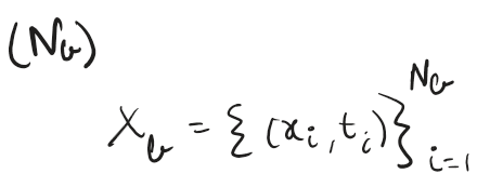
Let’s start with data loss, the network must anchor itself to the known universe. We provide it with a set of boundary points or initial conditions (Nb), these are the specific coordinates where we have actual sensor data or known physical constraints (u_true)

In this case we’re taking a Mean Squared Error (MSE) between the predicted and true values.

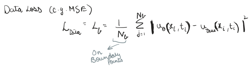
If we stopped here, we would just have a standard, data hungry neural network. It would perfectly memorize the boundary points but hallucinate wildly everywhere else.

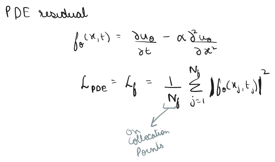
Now we introduce the governing physical law. In this case, we use the 1D Heat Equation as our residual, which dictates how temperature diffuses over space and time. In a perfect physical simulation, this equation must exactly equal zero.

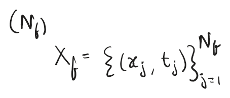
We evaluate this residual across a massive set of Collocation Points (Nf). These are data free coordinates randomly sampled from inside our physical domain. The network has no ground truth data here, but we force it to evaluate its own continuous derivatives using Automatic Differentiation.

The Data Loss and the Physics Loss operate on completely different scales and have completely different geometric landscapes.

Sometimes, the physics equation is incredibly complex to calculate, but memorizing the 5 sensor data points is easy. The network’s gradients will heavily prioritize dropping the Data Loss to zero, entirely ignoring the laws of physics. Other times, the network might find a trivial solution to the physics (like guessing the temperature is exactly 0 everywhere, making the PDE 0, satisfying the residual), ignoring the actual sensor data entirely.

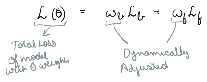
Hence we parameterize total loss using specific weights

We can set them to our desired behavior or could even adjust them dynamically, such that at every epoch, we force the network to respect the boundary data and the physical laws equally, guiding it safely to a converged, physically accurate simulation.

Optimization

To train the network, we must update our weights and biases (theta) such that the total loss goes to zero (L_theta). We do this by computing the gradient (g_t) of the loss function with respect to the weights .

This is standard in training any ML model, however for PINNs the nature of loss function is quite different warranting a different optimization approach

We decide to go two phased here, first using Adam (ADAptive Moment estimation) which is a first order optimizer, looking only at immediate scope of landscape.

Adam uses momentum and velocity, where momentum is exponentially decaying average of past gradients, physically, if the algorithm has been rolling down a steep hill for 100 steps, it builds up mathematical momentum. If it suddenly hits a small uphill bump (a local minimum), the momentum carries it right over the bump so it doesn’t get stuck.

Velocity is average squared of gradients. This acts as an adaptive brake. If the gradients suddenly become massive and chaotic (indicating the algorithm just walked off a cliff), v spikes, automatically shrinks the step size (eta) so the algorithm doesn’t fly off into infinity.
If the landscape flattens out, v shrinks, allowing the algorithm to confidently take massive strides.

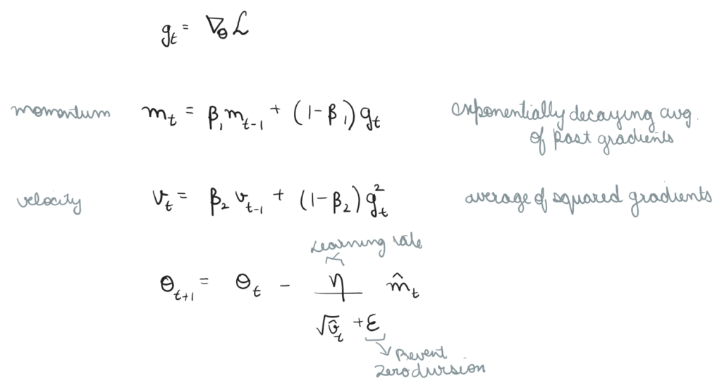
Adam is phenomenal at rapidly exploring rough terrain and finding the deepest valley. But once it gets to the bottom of that valley, it struggles to find the exact, pinpoint minimum. It bounces and oscillates violently around the bottom. And here comes the part 2 of our two phased approach.

Once Adam has safely navigated us to the bottom of the valley, we pause training and hand the neural network’s weights over to L-BFGS (Limited Memory Broyden Fletcher Goldfarb Shanno)

Where Adam only looks at the slope, L-BFGS looks at the entire landscape, it is a second order function

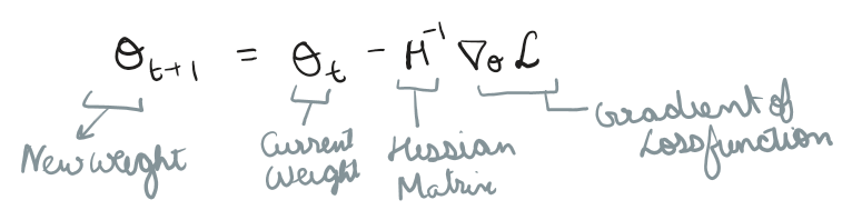
If a neural network has 10k weights, the Hessian is 10k x 10k, which means 100M second derivatives at every time step, which gets very compute intensive, to solve for memory we usually only look at last m steps, (usually 50 or 100) and uses those past gradients to efficiently approximate the inverse Hessian Matrix.

And then we iterate this process till we get desirable results or reach our number of epochs or early stopping conditions.

Conclusion

In Parts I, II, and III, we explored the classical analytical engine. We used characteristic equations, Laplace transforms, and state space matrices to perfectly decode isolated, linear systems. We saw how brilliant minds mathematically reverse engineered the physical world.

In Part IV, we confronted the chaotic reality of the real universe. When the physics became violently nonlinear, we abandoned exact equations and learned to discretize reality, using numerical solvers like RK45 and Finite Element Methods to chop time and space into computable, simulated fragments, leveraging the power of computers to solve complicated physics.

And now, with Physics Informed Neural Networks, we no longer have to choose between the rigorous, deterministic truth of classical calculus and the blazing, predictive speed of modern AI. By forcing a neural network to act as a continuous surrogate model, anchoring it with sparse data, and punishing it for violating the differential equations using Autodiff and two-phase optimization, we achieve something profound. We stop treating machine learning as a blind curve fitter. We can teach the machine the laws of thermodynamics, fluid dynamics, and orbital mechanics.

Whether we are attempting to forecast spatiotemporal Earth Observation data, model the thermal dynamics of a re entering spacecraft, or filter the noisy astrophysics of the cosmos, we now have the ultimate toolkit.

We have finally built a machine that sees the geometry of change exactly the way we do.

I wrote these series as a preface to some projects I am working on the side and as a reference for what’s to come next, hope it was detailed and comprehensive enough to outline the whole landscape and improve understanding.