It’s been a minute since my last post on data acquisition. Between a much needed vacation – trip to Italy and wrapping up my tap dance recital (because life exists outside of PyTorch!), sitting down to write about this project took a backseat, as this whole process is quite time consuming, believe it or not, and the charm kinda fades away after you’ve done the project, oh no my model is not near as accurate as I’d like but it met my first iteration standards and then kinda got pushed in the background as you probably saw in my differential equations series. Now that I’m finally getting around to documenting the model architecture, I realized I completely skipped the prequel – the data prep, which I actually built way back at the start of the project, so, well a while ago.
Before we get into U-Nets and loss functions, let’s quickly summarize how we wrangle the raw satellite data

Setup

I have described the sources available and provided their overview in the first post, in this post we assume we have the data downloaded as follows:

{REGION}/
├── GAUL/GAUL_{REGION}_boundary.geojson     # Administrative boundary (crop AOI)
├── S1/S1_{REGION}_S1_{YYYY-MM-DD}.tif      # Sentinel-1 VV + VH (master grid)
├── ENV/ENV_{REGION}_env_stack.tif          # Static environmental stack
├── HYDRO/HYDRO_MERIT_{REGION}_hydro_merit.tif
├── WEATHER/WEATHER_{REGION}_weather_1km_{YYYY-MM-DD}.tif
├── GFM_Benchmark_{REGION}/*{YYYYMMDD}*.tif   # GFM tiles (merged per date)
└── GloFAS_{REGION}/GLOFAS_{REGION}_{YYYY-MM-DD}.tif

I don’t use things like GloFAS and HYDRO but i do the data prep regardless.

Loading

We open our GeoTIFFs and crop it to the GAUL administrative boundary.

• Reproject the boundary to the raster CRS if needed
• Keep only polygons overlapping the raster bounds
• Apply a tiny geometry buffer (0.0001°) to avoid GDAL edge precision bugs
• Mask with all_touched=True so edge pixels are included
• Convert nodata to NaN and cast to float32

For S1, crop_to_aoi=True restricts the scene to the region of interest. The returned profile (transform, CRS, height, width) becomes the master grid.

Image Alignment

We force all disparate geospatial datasets to share the exact same pixel grid, dimensions, and Coordinate Reference System (CRS) as our master S1 imagery.

Every other raster is warped onto the S1 grid via rasterio.warp.reproject

We use a Resampling Algorithm based on the data, Nearest neighbor for env/gfm to protect categorical landcover classes which grabs the exact value of the single closest pixel without averaging and Bilinear Interpolation which calculates a weighted average of the 4 nearest pixels and creates smooth transitions for continuous data like rainfall or radar backscatter.

Additionally values below -9000 are treated as nodata and set to NaN

Global Stats

Before normalization, we scan a random subsample of ENV, WEATHER, and HYDRO GeoTIFFs (default 10 files, up to 100k pixels per band per file) and computes per-band 1st percentile, 99th percentile, and mean.

These stats help inspect the data and drive percentile-based scaling for elevation and hydro. They are computed once per region and reused for all dates.

Results are saved to stats_{REGION}.json (or stats.json for single-date tests).

• ENV band 4 (land cover) is skipped
• ENV elevation ignores values below -100 m (sensor noise)

Sanitization & Normalization

We handle each data source separately, because they’re obtained from different sources, measure different values and operate in different scales

For S1, we firstly remove the sensor noise, pixels below -50 dB → NaN (SAR noise floor), then filled as 0 after scaling. We use strict physical bounds instead of dataset stats because backscatter has well-known ranges:

• VV clipped to [-25, 0] dB → [0, 1]
• VH clipped to [-30, -5] dB → [0, 1]

Water acts as a specular reflector, bouncing radar pulses away from the sensor, resulting in extremely low backscatter (dark pixels, near -25 dB). Urban areas and rough vegetation cause double-bounce or volume scattering, resulting in high backscatter (bright pixels, near 0 dB)

For Weather, we have a few selected bands, which we scale as follows:

For GloFAS, even though we don’t use it, discharge clipped to [0, 1] by dividing by 2500 m³/s (empirical flood spike cap).

For GFM which is the primary supervised label, we binarize the data into flood and no flood:

• Valid pixels: not NaN and not 255
• Flood = any value > 0 → 1.0; otherwise 0.0

Cleaning up the Environment is multi step process, for the Continuous bands:

Land cover (band 5) is one-hot encoded into 11 channels (World Cover classes), essentially giving each World cover class its own binary channel.

For Hydro, its a single band scaled with global 1st/99th percentiles from scene stats. Again we don’t use this

Temporal Alignment

Environment is a static file but data like S1, GFM and weather is available on different timestamps, the details of which you can find in the data acquisition post.

We have already downloaded daily data, but we need to align these different modalities as they might not be for the same date

For GFM, we find all GFM tiles matching the date, merges them with rasterio.merge, writes a temporary GeoTIFF, aligns to master grid, then deletes the temp file.

For weather, we load the pre-aggregated GEE weather stack for the target date.

Then we match dates and align the data

Tiling

Instead of physically shattering the rasters into thousands of tiny files which causes massive disk I/O bottlenecks I implemented a virtual tiling strategy. The pipeline exports the full aligned scene as a single .npz file and generates a mathematical grid of 256×256 coordinates. Later, during the PyTorch DataLoader phase, the dataset dynamically crops these coordinates in memory and applies the 1% target rule, discarding unnecessary dry patches before they ever hit the GPU

We don’t tile/patch our data here exactly, but we create an outline for it, I wrote a helper function, build_tile_index, that acts as a mathematical cartographer. It iterates over the master height and width, stepping by a defined stride (256 pixels), and calculates the exact (x, y, w, h) bounding boxes for every possible non-overlapping patch in the scene.

S1 Labels – Optional

I optionally build a secondary label on S1 using otsu threshold and lee median filtering, it didn’t look that great so, i haven’t used it, and trained the model with GFM

It’s basically an auxiliary water mask built from raw S1 dB values (again not used as the primary training target – or anything right now – not unless I improve it):

1. Mask valid pixels (both bands > -50 dB)
2. Lee filter (7×7) to reduce speckle while preserving edges
3. Otsu threshold on high-variance edge pixels (top 10% local variance) for VV and VH, with fallbacks at -17.0 and -23.0 dB
4. Water if VV ≤ threshold or both bands are borderline below threshold
5. 3×3 median filter for spatial cleanup

Also produces s1_label_valid (where SAR data exists) and metadata: Otsu thresholds, positive pixel count, pos_weight for class imbalance.

Known limitations – Otsu fails on unimodal scenes, misses wind-roughened water, misclassifies radar shadows and smooth tarmac, and ignores double-bounce flooding in urban/forested areas.

--- S1 Label vs GFM Benchmark IoU ---
Valid Evaluation Pixels : 41132045
Intersection            : 429243
Union                   : 24371725
IoU Score               : 0.0176

Putting it Together

Pipeline

Then we sequence all our steps and create a pipeline, the final pipeline looks somewhat like:

For each target date, the pipeline:

1. Loads and normalizes S1; establishes master grid
2. Builds S1 labels
3. Loads static ENV + HYDRO (cached after first date in a region)
4. Loads and normalizes weather and GloFAS
5. Builds GFM mosaic and normalizes to binary mask
6. Loads S1 temporal lags (s1_t0 = current, s1_t-1, s1_t-2 from prior acquisitions in the sorted date inventory; zeros if unavailable)
7. Spatial masking: multiplies ENV, hydro, weather, glofas, and GFM tensors by s1_label_valid so invalid SAR pixels are zeroed consistently
8. Returns (tensors, tensors_selected, master_profile)

def process_date_pipeline(
    target_date: str, base_dir: str, region: str, 
    scene_stats: dict, static_cache=None, s1_lag_paths=None
):
    print(f"\n{'=' * 50}\nExecuting Pipeline for Target Date: {target_date}\n{'=' * 50}")
    
    paths = {
        "gaul": os.path.join(base_dir, "GAUL", f"GAUL_{region}_boundary.geojson"),
        "s1": os.path.join(base_dir, "S1", f"S1_{region}_S1_{target_date}.tif"),
        "env": os.path.join(base_dir, "ENV", f"ENV_{region}_env_stack.tif"),
        "hydro": os.path.join(base_dir, "HYDRO", f"HYDRO_MERIT_{region}_hydro_merit.tif"),
        "weather_dir": os.path.join(base_dir, "WEATHER"),
        "gfm_dir": os.path.join(base_dir, f"GFM_Benchmark_{region}"),
        "glofas_dir": os.path.join(base_dir, f"GloFAS_{region}"),
    }

    tensors = {}

    # 1. Core S1 (Load S1 and crop to GAUL)
    s1_raw, master_profile = load_and_crop_data(paths["s1"], paths["gaul"], crop_to_aoi=True)
    tensors["s1_raw"] = s1_raw
    tensors["s1"] = normalize_s1(s1_raw)
    print(f"  [OK] S1 loaded and normalized. Shape: {s1_raw.shape}")

    s1_lbl, s1_lbl_val, s1_lbl_meta = build_s1_label_from_raw(s1_raw)
    tensors.update({"s1_label": s1_lbl, "s1_label_valid": s1_lbl_val, "s1_label_meta": s1_lbl_meta})
    print(f"  [OK] S1 Labels generated (Otsu VV: {s1_lbl_meta['s1_otsu_vv']:.2f})")

    # 2. Static - Environment & Hydrology
    tensors.update(extract_static_context(paths, master_profile, scene_stats, static_cache))
    print(f"  [OK] Static ENV & HYDRO context loaded" + (" (from cache)" if static_cache else ""))

    # 3. Dynamic - Weather & GloFAS
    w_raw = process_daily_weather(target_date, paths["weather_dir"], region, master_profile)
    tensors["weather_raw"] = w_raw
    tensors["weather"] = normalize_weather(w_raw) if w_raw is not None else np.zeros((6, master_profile["height"], master_profile["width"]), dtype=np.float32)
    print(f"  [OK] Weather loaded and normalized. Shape: {w_raw.shape}")

    g_raw = process_daily_glofas(target_date, paths["glofas_dir"], region, master_profile)
    tensors["glofas_raw"] = g_raw
    if g_raw is not None:
        tensors["glofas"] = normalize_glofas(g_raw)  
        print(f"  [OK] GloFAS loaded and normalized. Shape: {g_raw.shape}")
    else:
        tensors["glofas"] = np.zeros((1, master_profile["height"], master_profile["width"]), dtype=np.float32)
        print(f"  [SKIP] GloFAS dummy initialized.")

    # 4. GFM Ground Truth
    gfm_mosaic = build_gfm_mosaic(target_date, paths["gfm_dir"], master_profile)
    tensors["gfm_raw"] = gfm_mosaic
    if gfm_mosaic is not None:
        tensors.update({
            "gfm_mask": normalize_gfm(gfm_mosaic),
            "gfm_valid": (~np.isnan(gfm_mosaic)).astype(np.float32),
            "gfm_missing": False
        })
        print(f"  [OK] GFM loaded and normalized. Shape: {gfm_mosaic.shape}")
    else:
        z_mask = np.zeros((1, master_profile["height"], master_profile["width"]), dtype=np.float32)
        tensors.update({"gfm_mask": z_mask.copy(), "gfm_valid": z_mask.copy(), "gfm_missing": True})
        print(f"  [SKIP] GFM dummy initialized")

    # 5. Temporal Lags
    tensors["s1_t0"] = tensors["s1"]
    zlag = np.zeros_like(tensors["s1"], dtype=np.float32)
    
    p2 = s1_lag_paths[0] if s1_lag_paths and len(s1_lag_paths) > 0 else None
    p1 = s1_lag_paths[1] if s1_lag_paths and len(s1_lag_paths) > 1 else None
    
    lag2, lag1 = load_s1_lag_normalized(p2, master_profile), load_s1_lag_normalized(p1, master_profile)
    tensors["s1_t-2"] = lag2 if lag2 is not None else zlag.copy()
    tensors["s1_t-1"] = lag1 if lag1 is not None else zlag.copy()
    print(f"  [OK] s1 Lag loaded and normalized")

    # 6. Apply Universal Spatial Masking
    mask = tensors["s1_label_valid"]
    _mask_keys = [
        *ENV_CONTINUOUS_BAND_KEYS,
        "env_landcover",
        "hydro",
        "weather",
        "glofas",
        "gfm_mask",
        "gfm_valid",
    ]
    for key in _mask_keys:
        tensors[key] = tensors[key] * mask

    # 7. Final Selection
    selected_keys = [
        "s1",
        "s1_label",
        *ENV_CONTINUOUS_BAND_KEYS,
        "env_landcover",
        "hydro",
        "weather",
        "glofas",
        "gfm_mask",
        "s1_label_valid",
        "gfm_valid",
        "s1_t0",
        "s1_t-1",
        "s1_t-2",
    ]
    tensors_selected = {k: tensors[k] for k in selected_keys}

    return tensors, tensors_selected, master_profile

def process_date_pipeline(
    target_date: str, base_dir: str, region: str, 
    scene_stats: dict, static_cache=None, s1_lag_paths=None
):
    print(f"\n{'=' * 50}\nExecuting Pipeline for Target Date: {target_date}\n{'=' * 50}")
    
    paths = {
        "gaul": os.path.join(base_dir, "GAUL", f"GAUL_{region}_boundary.geojson"),
        "s1": os.path.join(base_dir, "S1", f"S1_{region}_S1_{target_date}.tif"),
        "env": os.path.join(base_dir, "ENV", f"ENV_{region}_env_stack.tif"),
        "hydro": os.path.join(base_dir, "HYDRO", f"HYDRO_MERIT_{region}_hydro_merit.tif"),
        "weather_dir": os.path.join(base_dir, "WEATHER"),
        "gfm_dir": os.path.join(base_dir, f"GFM_Benchmark_{region}"),
        "glofas_dir": os.path.join(base_dir, f"GloFAS_{region}"),
    }

    tensors = {}

    # 1. Core S1 (Load S1 and crop to GAUL)
    s1_raw, master_profile = load_and_crop_data(paths["s1"], paths["gaul"], crop_to_aoi=True)
    tensors["s1_raw"] = s1_raw
    tensors["s1"] = normalize_s1(s1_raw)
    print(f"  [OK] S1 loaded and normalized. Shape: {s1_raw.shape}")

    s1_lbl, s1_lbl_val, s1_lbl_meta = build_s1_label_from_raw(s1_raw)
    tensors.update({"s1_label": s1_lbl, "s1_label_valid": s1_lbl_val, "s1_label_meta": s1_lbl_meta})
    print(f"  [OK] S1 Labels generated (Otsu VV: {s1_lbl_meta['s1_otsu_vv']:.2f})")

    # 2. Static - Environment & Hydrology
    tensors.update(extract_static_context(paths, master_profile, scene_stats, static_cache))
    print(f"  [OK] Static ENV & HYDRO context loaded" + (" (from cache)" if static_cache else ""))

    # 3. Dynamic - Weather & GloFAS
    w_raw = process_daily_weather(target_date, paths["weather_dir"], region, master_profile)
    tensors["weather_raw"] = w_raw
    tensors["weather"] = normalize_weather(w_raw) if w_raw is not None else np.zeros((6, master_profile["height"], master_profile["width"]), dtype=np.float32)
    print(f"  [OK] Weather loaded and normalized. Shape: {w_raw.shape}")

    g_raw = process_daily_glofas(target_date, paths["glofas_dir"], region, master_profile)
    tensors["glofas_raw"] = g_raw
    if g_raw is not None:
        tensors["glofas"] = normalize_glofas(g_raw)  
        print(f"  [OK] GloFAS loaded and normalized. Shape: {g_raw.shape}")
    else:
        tensors["glofas"] = np.zeros((1, master_profile["height"], master_profile["width"]), dtype=np.float32)
        print(f"  [SKIP] GloFAS dummy initialized.")

    # 4. GFM Ground Truth
    gfm_mosaic = build_gfm_mosaic(target_date, paths["gfm_dir"], master_profile)
    tensors["gfm_raw"] = gfm_mosaic
    if gfm_mosaic is not None:
        tensors.update({
            "gfm_mask": normalize_gfm(gfm_mosaic),
            "gfm_valid": (~np.isnan(gfm_mosaic)).astype(np.float32),
            "gfm_missing": False
        })
        print(f"  [OK] GFM loaded and normalized. Shape: {gfm_mosaic.shape}")
    else:
        z_mask = np.zeros((1, master_profile["height"], master_profile["width"]), dtype=np.float32)
        tensors.update({"gfm_mask": z_mask.copy(), "gfm_valid": z_mask.copy(), "gfm_missing": True})
        print(f"  [SKIP] GFM dummy initialized")

    # 5. Temporal Lags
    tensors["s1_t0"] = tensors["s1"]
    zlag = np.zeros_like(tensors["s1"], dtype=np.float32)
    
    p2 = s1_lag_paths[0] if s1_lag_paths and len(s1_lag_paths) > 0 else None
    p1 = s1_lag_paths[1] if s1_lag_paths and len(s1_lag_paths) > 1 else None
    
    lag2, lag1 = load_s1_lag_normalized(p2, master_profile), load_s1_lag_normalized(p1, master_profile)
    tensors["s1_t-2"] = lag2 if lag2 is not None else zlag.copy()
    tensors["s1_t-1"] = lag1 if lag1 is not None else zlag.copy()
    print(f"  [OK] s1 Lag loaded and normalized")

    # 6. Apply Universal Spatial Masking
    mask = tensors["s1_label_valid"]
    _mask_keys = [
        *ENV_CONTINUOUS_BAND_KEYS,
        "env_landcover",
        "hydro",
        "weather",
        "glofas",
        "gfm_mask",
        "gfm_valid",
    ]
    for key in _mask_keys:
        tensors[key] = tensors[key] * mask

    # 7. Final Selection
    selected_keys = [
        "s1",
        "s1_label",
        *ENV_CONTINUOUS_BAND_KEYS,
        "env_landcover",
        "hydro",
        "weather",
        "glofas",
        "gfm_mask",
        "s1_label_valid",
        "gfm_valid",
        "s1_t0",
        "s1_t-1",
        "s1_t-2",
    ]
    tensors_selected = {k: tensors[k] for k in selected_keys}

    return tensors, tensors_selected, master_profile

Export

I also have an export function, which writes data in a specific format:

Write two files per sample:

selected_{REGION}_{YYYY-MM-DD}.npz

• Float32 for continuous tensors
• Uint8 for masks, labels, and validity channels
• ENV continuous bands stored as separate keys (env_elevation, …) not a merged stack

selected_{REGION}_{YYYY-MM-DD}.json

Metadata includes:

• schema_version, sample_id, region, date, horizon, split
• shape_by_key — channel/spatial dimensions per array
• crs, transform — georeferencing from master S1 profile
• tile_grid — 256×256 non-overlapping tile index for downstream patching
• lag_keys, s1_lag_dates
• pos_weight, positive_ratio, gfm_missing
• include_env_continuous — optional band filtering at export time

After running the notebook, the prepared dataset lives under EXPORT_DIR:

prepared/
├── selected_Ottawa_2019-04-08.npz
├── selected_Ottawa_2019-04-08.json
├── selected_Ottawa_2019-04-13.npz
├── selected_Ottawa_2019-04-13.json
└── ...

Each pair is one georeferenced scene at S1 resolution (~6399 × 12333 pixels in the Ottawa example), with:

• All modalities aligned and normalized
• GFM binary flood mask as the supervised target
• Validity masks for SAR and GFM coverage
• Three timesteps of normalized S1 (current + two lags)
• JSON metadata for tiling, class weights, and provenance

Batch

I run this function in batch using a ThreadPoolExecutor, I have a small sample to this basic multithreading works for me at this stage.

The production run loop:

1. For each region in REGIONS
2. Compute and save stats_{REGION}.json
3. Inventory all S1 dates; optionally filter by cutoff date
4. Build S1 lag path maps (build_s1_lag_maps)
5. Process the first date sequentially to populate the static ENV/HYDRO cache
6. Process remaining dates in parallel (ThreadPoolExecutor, default 4 workers) with the shared static cache

Each worker calls process_date_pipeline → export_prepared_sample, a log looks somewhat like:

==================================================
Executing Pipeline for Target Date: 2019-05-07
==================================================
  [OK] S1 loaded and normalized. Shape: (2, 6399, 12333)
  [OK] S1 Labels generated (Otsu VV: -10.04)
  [OK] Static ENV & HYDRO context loaded (from cache)
Processing weather for 2019-05-07 : D:\Projects\datasets\raw\Ottawa\WEATHER\WEATHER_Ottawa_weather_1km_2019-05-07.tif
  [OK] Weather loaded and normalized. Shape: (6, 6399, 12333)
  [WARN] GloFAS missing for 2019-05-07; returning empty tensor.
  [SKIP] GloFAS dummy initialized.
Building GFM mosaic for 2019-05-07 : 4 tiles
[EXPORT] Saved selected_Ottawa_2019-04-13.npz and .json

Analysis & Checks

valid mask: s1_label_valid & gfm_valid, coverage=34.46% of grid (5452658 px)

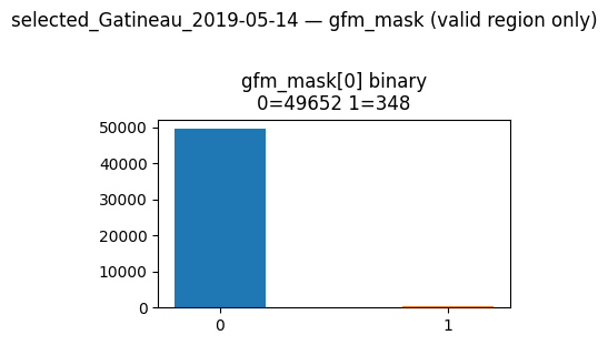
Look at the distribution of the GFM supervised target mask. Even after applying spatial subsetting, the massive spike at 0.0 (dry land) completely dwarfs the microscopic blip at 1.0 (flood water). This single plot is a stark visual warning of what’s to come.

s1: tensor (2, 2522, 6274)

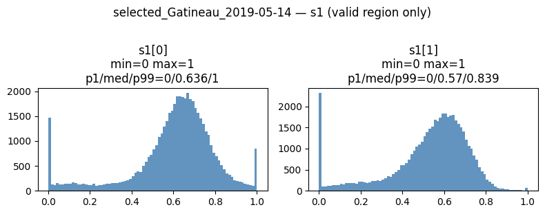
You can clearly see the data has been cleanly bound between 0.0 and 1.0. By physically clipping the VV backscatter to a [-25, 0] dB range prior to scaling, we preserved the natural bimodal spread of the radar returns (separating the dark, specular water reflections from the bright, double-bounce urban reflections) while entirely eliminating the sensor noise floor.

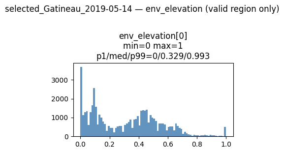
env_elevation: tensor (1, 2522, 6274)

env_water_occ: tensor (1, 2522, 6274)

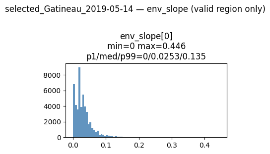
env_slope: tensor (1, 2522, 6274)

env_hand: tensor (1, 2522, 6274)

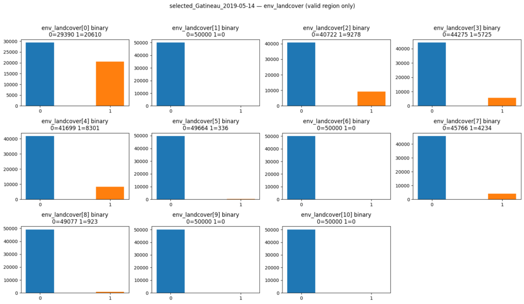
env_landcover: tensor (11, 2522, 6274)

weather: tensor (6, 2522, 6274)

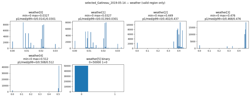
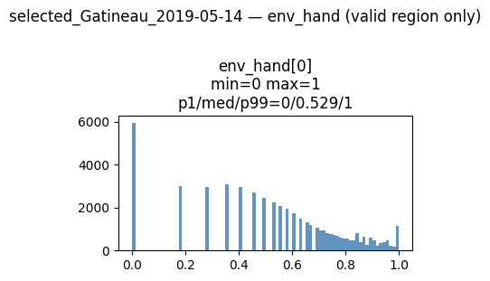
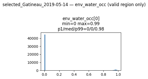
The continuous environmental and weather bands (Elevation, Slope, Precipitation, Soil Moisture) are all operating on completely different physical scales (degrees, millimeters, Kelvin). Our percentile-based and static normalization pipelines successfully squeezed these disparate metrics into a uniform [0, 1] tensor space without destroying the long-tail anomalies like the extreme precipitation spikes you can see in the 1-day and 3-day weather lags.

The purpose of above plots is to check shape of tensors and normalization, the final list of features will be discussed briefly in my next post

Below is the statistical summary of our data (1 .npz file):

==================================================
TENSOR STATISTICAL SUMMARY
==================================================
s1_raw          | Shape: (2, 6399, 12333) | Valid: 52.1% | Min: -65.26 | Max: 29.05 | Mean: -16.35
s1              | Shape: (2, 6399, 12333) | Valid: 100.0% | Min: 0.00 | Max: 1.00 | Mean: 0.23
s1_label        | Shape: (1, 6399, 12333) | Valid: 100.0% | Min: 0.00 | Max: 1.00 | Mean: 0.31
s1_label_valid  | Shape: (1, 6399, 12333) | Valid: 100.0% | Min: 0.00 | Max: 1.00 | Mean: 0.52
env_raw         | Shape: (5, 6399, 12333) | Valid: 42.1% | Min: 0.00 | Max: 173.00 | Mean: 33.70
env_elevation   | Shape: (1, 6399, 12333) | Valid: 100.0% | Min: 0.00 | Max: 1.00 | Mean: 0.23
env_slope       | Shape: (1, 6399, 12333) | Valid: 100.0% | Min: 0.00 | Max: 0.64 | Mean: 0.02
env_hand        | Shape: (1, 6399, 12333) | Valid: 100.0% | Min: 0.00 | Max: 1.00 | Mean: 0.24
env_water_occ   | Shape: (1, 6399, 12333) | Valid: 100.0% | Min: 0.00 | Max: 0.99 | Mean: 0.02
env_landcover   | Shape: (11, 6399, 12333) | Valid: 100.0% | Min: 0.00 | Max: 1.00 | Mean: 0.05
hydro_raw       | Shape: (1, 6399, 12333) | Valid: 52.1% | Min: 0.00 | Max: 193e+9| Mean: 779e+8
hydro           | Shape: (1, 6399, 12333) | Valid: 100.0% | Min: 0.00 | Max: 1.00 | Mean: 0.21
weather_raw     | Shape: (6, 6399, 12333) | Valid: 52.0% | Min: -0.00 | Max: 274.39 | Mean: 77.02
weather         | Shape: (6, 6399, 12333) | Valid: 100.0% | Min: 0.00 | Max: 0.48 | Mean: 0.15
glofas          | Shape: (1, 6399, 12333) | Valid: 100.0% | Min: 0.00 | Max: 0.00 | Mean: 0.00
gfm_raw         | Shape: (1, 6399, 12333) | Valid: 100.0% | Min: 0.00 | Max: 255.00 | Mean: 46.40
gfm_mask        | Shape: (1, 6399, 12333) | Valid: 100.0% | Min: 0.00 | Max: 1.00 | Mean: 0.01
gfm_valid       | Shape: (1, 6399, 12333) | Valid: 100.0% | Min: 0.00 | Max: 1.00 | Mean: 0.52
s1_t0           | Shape: (2, 6399, 12333) | Valid: 100.0% | Min: 0.00 | Max: 1.00 | Mean: 0.23
s1_t-2          | Shape: (2, 6399, 12333) | Valid: 100.0% | Min: 0.00 | Max: 0.00 | Mean: 0.00
s1_t-1          | Shape: (2, 6399, 12333) | Valid: 100.0% | Min: 0.00 | Max: 0.00 | Mean: 0.00