We’ve sourced the multi-modal satellite data, cleaned it and created a tensor pipeline, and dissected the mathematical morality of imbalanced loss functions. Now we dive into the core.

Load Data & Config

We load in the data we prepared in the previous post and bind different channels, create tensors, split data in traing test and val, here is a sample of how the data looks for one file:

The following image shows our two S1 bands (primary feature – radar image), the GFM labels (also displayed, but not used are the manually created S1 labels)

Here is another example with more layers visualized:

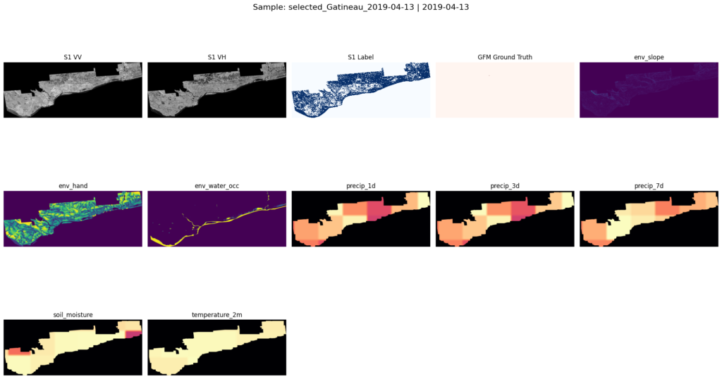
For more details please refer to data acquisition and data preparation pipelines.

Here is the config and layers we used in this run:

INCLUDE_ENV = {
    "env_elevation": False,
    "env_slope": True,
    "env_hand": True,
    "env_water_occ": True,
}
INCLUDE_S1_LAGS = {
    "s1_t-1": True, 
    "s1_t-2": True
}
INCLUDE_WEATHER = {
    "precip_1d": True,
    "precip_3d": True,
    "precip_7d": True,
    "soil_moisture": True,
    "temperature_2m": True,
    "total_evaporation": False,
}

INCLUDE_ENV_LANDCOVER = False
INCLUDE_HYDRO = False
INCLUDE_GLOFAS = False

Create Patches

Full satellite scenes are massively high-resolution, far too large to feed into a U-Net at once without triggering instant Out-Of-Memory (OOM) errors on the GPU. Training requires fixed spatial windows (in my case, PATCH_SIZE, 256×256 pixels)

However, because floods are rare anomalies (often making up <1% of a scene), a naive sliding window approach would generate thousands of patches containing nothing but dry land. The network would overfit to the background class immediately. So, there is a little bit of thought involved in this patching process.

Our patching pipeline is two phased:

The Manifest (Planning Phase): A spatial cartographer that calculates precise (y, x) bounding box coordinates to guarantee a specific statistical mix of flooded vs. dry land. so i can save it over the runs for consistency without bloating the space with both patches and scenes.

The Dataset (Loading Phase): The PyTorch DataLoader that physically crops the tensors at those coordinates during the training loop. Hence patches essentially created when the loader is called.

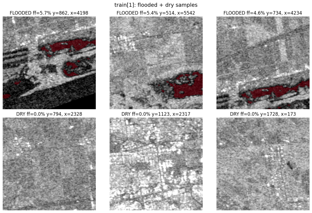
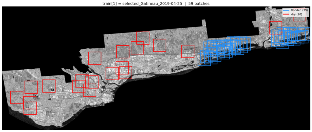
Firstly we build a patch manifest – this is essentially the planning phase, we pick (y, x) top-left corners per scene so the batch mix matches PATCH_QUOTAS (mostly “some flood”, some dry).

Config

Here is our patch config for the run:

PATCH_TARGET = "gfm_mask"
PATCH_SIZE = 256
PATCH_VALID_FRACTION = 0.90
PATCH_MAX_IOU = 0.50
TRAIN_PATCHES_PER_SCENE = 100
PATCH_QUOTAS = (
    (0.7, 0.01, None),    # 70% of patches MUST have at least 1% flood
    (0.1, 0.015, None),   # 10% of patches MUST have at least 1.5% flood
    (0.2, 0.00, 0.00),    # 20% of patches MUST be completely dry (0% flood)
)

We define a Patch Quota, with a per-scene patch mix with share, min_flood_frac, max_flood_frac. The shares should sum to 1 and flood fraction = flooded valid pixels / all valid pixels in the patch, we use max_flood_frac=None for no upper ca[ and use max=0.0 with min=0.0 for dry-only patches

For each scene, we fill each quota bucket by anchoring on label pixels (np.argwhere), then placing a PATCH_SIZE window around a random anchor. Flood buckets anchor on flooded valid pixels; the dry bucket anchors on valid non-flood pixels (uniform random fallback if none).

• For every scene – we do lazy loading in RAM, load the labels and only work with valid data
• We get the spatial bounds of the scene and flooded, not flooded pixel coordinates
• Then we proceed to full fill our set patch quotas
• We reject a patch if
  • too many invalid pixels (PATCH_VALID_FRACTION),
  • it overlaps an already chosen window (PATCH_MAX_IOU),
  • its flood fraction (flooded valid pixels ÷ all valid pixels) is outside the bucket’s min/max

Patch Search

For every scene,

• We take in the scene (pool), h and w and size
• Reject creating patches if no flood pixels in the scene
• Uniformly samples exactly one pixel coordinate pair from the valid pool to act as the anchor `(cy, cx)`
• Valid patch range for the anchor
  – `bottom = cy – patch_size + 1`
  – `top = min(cy, h – patch_size)`
  – `left = cx – patch_size + 1`
  – `right = min(cx, h – patch_size)`
• We reject if image is smaller than desired patch

Quota

Then we check quota validity, by evaluating the actual pixel contents of the proposed window to ensure it isn’t filled with “nodata” padding and that it matches the flood percentage required by the current quota bucket :

• We take in the full array (labels, valid pixels) & min-max flood threshold
• If no valid pixels in the window less than minimum threshold i.e. `PATCH_VALID_FRACTION`, reject the patch
• Create label patch window from top left anchors `(y,x)`
• Isolate only the valid pixels using boolean indexing
• Calculate the mean of valid labels in the patch
• Rejects if mean or flood fraction of patch defines bounds of min-max flood threshold

Overlap

Then we proceed to evaluate spatial overlap for our patches and reject patches which overlap more than desired fraction, to guarantee that the model does not train on the same geographic features repeatedly, we do this by calculating the Intersection over Union (IoU) between a proposed bounding box and all previously selected boxes 

• Take candidate coordinates `(y, x)` and a list of already selected chosen coordinates
• Iterate over every top-left coordinate pair previously approved for the current scene `(py, px)`
• Calculate the height and width intersection (ih, iw) – `Overlap = Bottom – Top = [min(y, py) + patch_size] – max(y, py)`
• Calculate area of intersect – `ih * iw`
• Apply the IOU threshold – Area_Intersection / Area_Union = intersection / ( patch1(h*w) + patch2(h*w) – intersection)

Then we define another dataset function which is essentially the loading phase, we crop inputs/labels at those corners and return (spatial, weather, label, valid), then we just wrap the dataset in a PyTorch DataLoader.

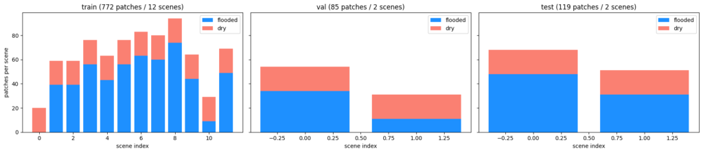
Here is the patch summary of the data we used and the config we described:

Features / Input

Above is the patch summary and the split details, each patch has multiple spatial channels:

spatial input: (32, 9, 256, 256)

And because of the nature of the model we’re using (Film UNet described in the next section) – we provide weather as linear modulation layer

weather vec: (32, 5)

Here is how a patch can look like:

  0  VV                            shape=(256, 256)  min=0  max=1  mean=0.399873
  1  VH                            shape=(256, 256)  min=0  max=1  mean=0.352138
  2  s1_t-1_VV                     shape=(256, 256)  min=0  max=1  mean=0.460086
  3  s1_t-1_VH                     shape=(256, 256)  min=0  max=1  mean=0.384164
  4  s1_t-2_VV                     shape=(256, 256)  min=0  max=1  mean=0.437939
  5  s1_t-2_VH                     shape=(256, 256)  min=0  max=1         mean=0.37158
  6  env_slope                     shape=(256, 256)  min=0  max=0.236625  mean=0.0237011
  7  env_hand                      shape=(256, 256)  min=0  max=1         mean=0.290433
  8  env_water_occ                 shape=(256, 256)  min=0  max=0.97      mean=0.232344

Model

If we were only looking at satellite imagery, a standard Convolutional Neural Network (CNN) like a U-Net would be perfectly sufficient. U-Nets are the gold standard for semantic segmentation because their encoder-decoder structure (with skip connections) captures both deep, abstract context and high-resolution spatial boundaries.

Convolutional Neural Networks (CNNs) like the U-Net love 2D grids (images). But weather data like 3 day precipitation accumulation or soil moisture is coarser and better as a 1D vector.

The naive approach is to simply tile the 1-dimensional weather data across the entire 256×256 image grid and concatenate it as an extra channel. However, this is computationally wasteful, heavily inflates the parameter count of the first convolution layer, and forces a spatial network to learn global context through a localized lens.

Instead of forcing the weather into the image, we use FiLM. Developed originally for visual reasoning tasks, FiLM allows a network to modulate its spatial feature maps based on external conditioning data.

I wrote about it before here, but I’ll discuss it briefly in this post as well.

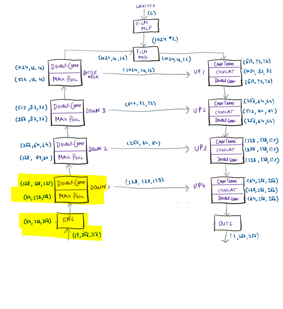
While the spatial input goes in through a standard input layer, in our case we have a batch of 32 and we chose to go ahead with only 9 channels right now, not 17, the bulk was landcover OHE channels which were not helping our model, so I decided to remove them for noe and inspect later.

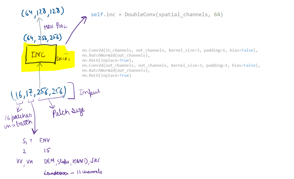
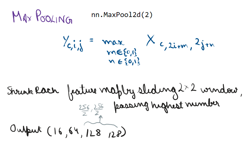
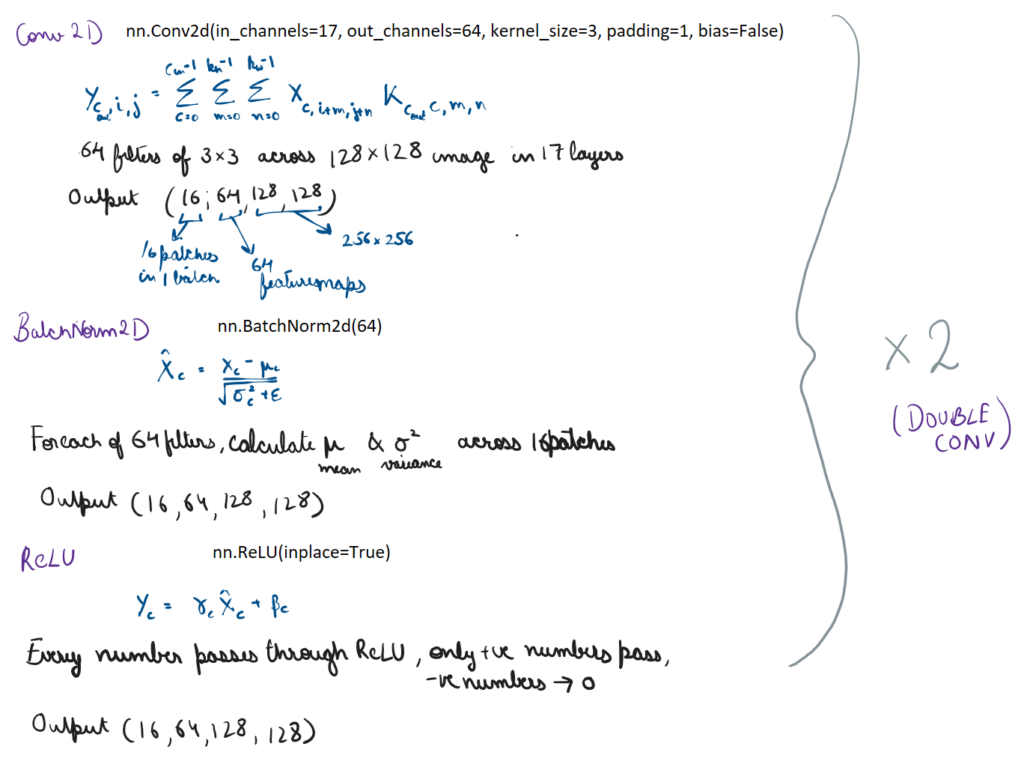
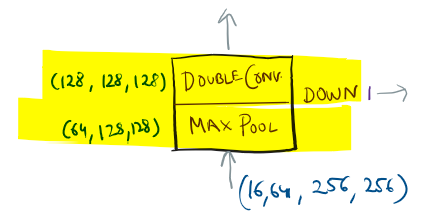
Then we have a standard double convolution block, you might be familiar with it already, 4 of these make the encoder part of our UNet

Before the weather data ever touches the image, it passes through its own isolated network branch. The 6-channel weather vector is fed into a simple Multi-Layer Perceptron (MLP). This “tabular encoder” compresses the raw meteorological values into a dense embedding, capturing the non-linear relationship between things like 7-day cumulative rainfall and current soil moisture.

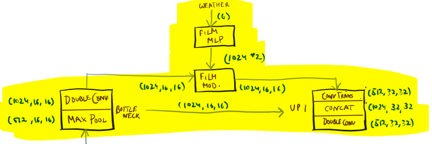
Think of it like a volume knob. Based on how heavily it rained (the weather vector), a Multi-Layer Perceptron (MLP) generates two scalars: gamma (scale) and beta (shift). It then applies an affine transformation to the spatial feature maps coming out of the U-Net convolutions

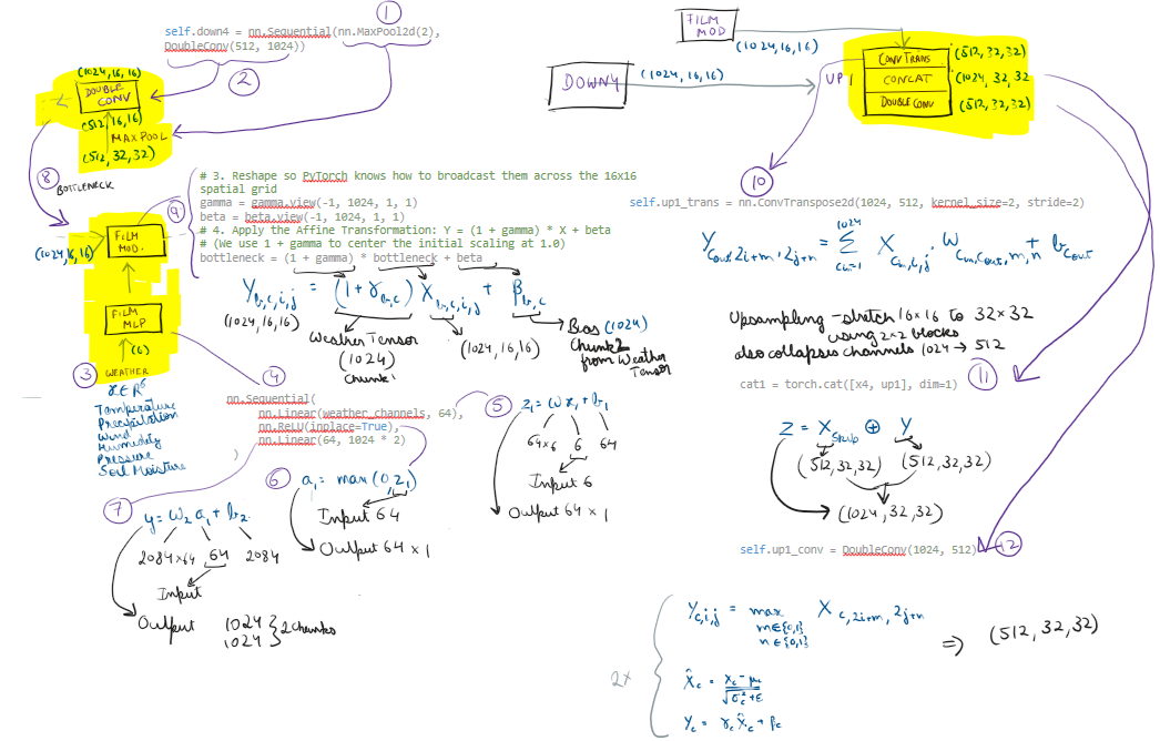
And although a bit rough, this is how the data flows:

Since floods are extremely rare < 1% pixels, we experimented with different loss functions you can read about them in detail here. We use the Focal Tversky Loss, you can even find the implementation in the mentioned post.

class FocalTverskyLoss(nn.Module):

  def __init__(
    self,
    focal_alpha: float = 0.25,      # focal class weight on positive pixels
    focal_gamma: float = 2.0,      # down-weight easy pixels: (1 - pt)^gamma
    tversky_alpha: float = 0.3,    # FP cost in Tversky denominator
    tversky_beta: float = 0.7,     # FN cost (β > α → recall-friendly)
    smooth: float = 1e-5,          # epsilon - to prevent division by 0
    tversky_weight: float = 1.0,
  ):
    super().__init__()
    # focal loss
    # alpha indicates class weight to positive class, gamma is the modulating factor
    self.focal_alpha, self.focal_gamma = focal_alpha, focal_gamma
    # tversky loss
    # beta = 0.8, alpha = 0.2  - penalizes FN 4x times more than FP
    self.tversky_alpha, self.tversky_beta = tversky_alpha, tversky_beta
    # smooth - epsilon - to prevent division by 0
    self.smooth, self.tversky_weight = smooth, tversky_weight

  def forward(self, logits, targets, valid_mask=None):
    #extract valid area to ignore void pixels
    m = torch.ones_like(targets) if valid_mask is None else valid_mask.float()
    #total number of pixels (valid)
    n = m.sum() + self.smooth  

    # --- Focal: batch-level pos_weight in BCE, then (1-pt)^gamma focusing ---
    # with torch.no_grad():
      # TP count
      # pos = (targets * m).sum()
      # TN count
      # neg = ((1 - targets) * m).sum()
      # dynamic ratio of positive to negative  (capped at 50)
      # pos_w = (neg / (pos + self.smooth)).clamp(1.0, 50.0)  # rare-flood upweight
    # calculate BCE 
    # bce = F.binary_cross_entropy_with_logits(logits, targets, reduction="none", pos_weight=pos_w)
    bce_unweighted = F.binary_cross_entropy_with_logits(logits, targets, reduction="none")
    pt = torch.exp(-bce_unweighted)
    # static alpha balancing map
    alpha_t = self.focal_alpha * targets + (1.0 - self.focal_alpha) * (1.0 - targets)
    # Focal formula
    # focal = (w * (1 - pt).pow(self.focal_gamma) * bce_unweighted * m).sum() / n
    focal_map = alpha_t * (1.0 - pt).pow(self.focal_gamma) * bce_unweighted
    focal = (focal_map * m).sum() / n

    # --- Tversky: soft tp/fp/fn per sample, then mean(1 - index) ---
    # Converts raw logits to probabilities and zeroes out invalid pixels
    p = (torch.sigmoid(logits) * m).flatten(1)
    # Flatten Ground Truth
    t = (targets * m).flatten(1)
    tp = (p * t).sum(1)
    fp = (p * (1 - t)).sum(1)
    fn = ((1 - p) * t).sum(1)
    # Tversky Formula
    tversky = 1 - (tp + self.smooth) / (tp + self.tversky_alpha * fp + self.tversky_beta * fn + self.smooth)
    # Averages the Tversky scores across the batch and adds the Focal loss
    return focal + self.tversky_weight * tversky.mean()

class FocalTverskyLoss(nn.Module):

  def __init__(
    self,
    focal_alpha: float = 0.25,      # focal class weight on positive pixels
    focal_gamma: float = 2.0,      # down-weight easy pixels: (1 - pt)^gamma
    tversky_alpha: float = 0.3,    # FP cost in Tversky denominator
    tversky_beta: float = 0.7,     # FN cost (β > α → recall-friendly)
    smooth: float = 1e-5,          # epsilon - to prevent division by 0
    tversky_weight: float = 1.0,
  ):
    super().__init__()
    # focal loss
    # alpha indicates class weight to positive class, gamma is the modulating factor
    self.focal_alpha, self.focal_gamma = focal_alpha, focal_gamma
    # tversky loss
    # beta = 0.8, alpha = 0.2  - penalizes FN 4x times more than FP
    self.tversky_alpha, self.tversky_beta = tversky_alpha, tversky_beta
    # smooth - epsilon - to prevent division by 0
    self.smooth, self.tversky_weight = smooth, tversky_weight

  def forward(self, logits, targets, valid_mask=None):
    #extract valid area to ignore void pixels
    m = torch.ones_like(targets) if valid_mask is None else valid_mask.float()
    #total number of pixels (valid)
    n = m.sum() + self.smooth  

    # --- Focal: batch-level pos_weight in BCE, then (1-pt)^gamma focusing ---
    # with torch.no_grad():
      # TP count
      # pos = (targets * m).sum()
      # TN count
      # neg = ((1 - targets) * m).sum()
      # dynamic ratio of positive to negative  (capped at 50)
      # pos_w = (neg / (pos + self.smooth)).clamp(1.0, 50.0)  # rare-flood upweight
    # calculate BCE 
    # bce = F.binary_cross_entropy_with_logits(logits, targets, reduction="none", pos_weight=pos_w)
    bce_unweighted = F.binary_cross_entropy_with_logits(logits, targets, reduction="none")
    pt = torch.exp(-bce_unweighted)
    # static alpha balancing map
    alpha_t = self.focal_alpha * targets + (1.0 - self.focal_alpha) * (1.0 - targets)
    # Focal formula
    # focal = (w * (1 - pt).pow(self.focal_gamma) * bce_unweighted * m).sum() / n
    focal_map = alpha_t * (1.0 - pt).pow(self.focal_gamma) * bce_unweighted
    focal = (focal_map * m).sum() / n

    # --- Tversky: soft tp/fp/fn per sample, then mean(1 - index) ---
    # Converts raw logits to probabilities and zeroes out invalid pixels
    p = (torch.sigmoid(logits) * m).flatten(1)
    # Flatten Ground Truth
    t = (targets * m).flatten(1)
    tp = (p * t).sum(1)
    fp = (p * (1 - t)).sum(1)
    fn = ((1 - p) * t).sum(1)
    # Tversky Formula
    tversky = 1 - (tp + self.smooth) / (tp + self.tversky_alpha * fp + self.tversky_beta * fn + self.smooth)
    # Averages the Tversky scores across the batch and adds the Focal loss
    return focal + self.tversky_weight * tversky.mean()

Training a model on extreme class imbalance with a rational loss function like Focal-Tversky is notoriously unstable. For memory, we run the data using PyTorch’s Automatic Mixed Precision (AMP), running the forward pass in 16-bit floats. The limited numerical range and small loss values for detecting < 1% data’s boundary detection, we wrapped the loss in a grad scaler, mathematically inflating the loss before back prop.

scaler = torch.amp.GradScaler("cuda", enabled=use_amp)

with torch.amp.autocast("cuda", enabled=use_amp):
    loss = crit(model(spatial, weather), mask, valid_mask)
    
scaler.scale(loss).backward()
scaler.step(opt)
scaler.update()

scaler = torch.amp.GradScaler("cuda", enabled=use_amp)

with torch.amp.autocast("cuda", enabled=use_amp):
    loss = crit(model(spatial, weather), mask, valid_mask)
    
scaler.scale(loss).backward()
scaler.step(opt)
scaler.update()

For optimizer, we used adam with cosine annealing LR since we have Tversky coupled in the loss function, making it non convex, we need to have a cosine LR scheduler which allows the learning rate to start high (to escape bad initialization pockets) and smoothly decay to a specified minimum, so that we don’t get stuck in a plateau when predicting zeroes everywhere and can find a global minima

opt = torch.optim.Adam(model.parameters(), lr=LEARNING_RATE)
sched = torch.optim.lr_scheduler.CosineAnnealingLR(opt, T_max=max(EPOCHS, 1), eta_min=LR_MIN)

opt = torch.optim.Adam(model.parameters(), lr=LEARNING_RATE)
sched = torch.optim.lr_scheduler.CosineAnnealingLR(opt, T_max=max(EPOCHS, 1), eta_min=LR_MIN)

Instead of tracking loss, I evaluated the network at the end of every epoch by computing a continuous Precision-Recall (PR) Curve. The validation loop calculates the exact F1 score across a linear grid of 99 different probability thresholds. The Early Stopping callback is strictly tied to the optimal F1 score instead of val loss or val accuracy.

# Save if PR-optimal F1 improves AND the model actually found True Positives. 
f1_up = (val_f1 > best_f1 + 1e-6) and (tp > 0)
loss_up = (avg_val < best_loss - 1e-6)

# If early training F1 is stuck at 0, allow loss improvement to guide it.
if f1_up or (loss_up and best_f1 <= 0.0):
    best_f1 = val_f1
    torch.save(checkpoint, BEST_MODEL_PATH)

# Save if PR-optimal F1 improves AND the model actually found True Positives. 
f1_up = (val_f1 > best_f1 + 1e-6) and (tp > 0)
loss_up = (avg_val < best_loss - 1e-6)

# If early training F1 is stuck at 0, allow loss improvement to guide it.
if f1_up or (loss_up and best_f1 <= 0.0):
    best_f1 = val_f1
    torch.save(checkpoint, BEST_MODEL_PATH)

To begin with, we just started with 20 epochs and got:

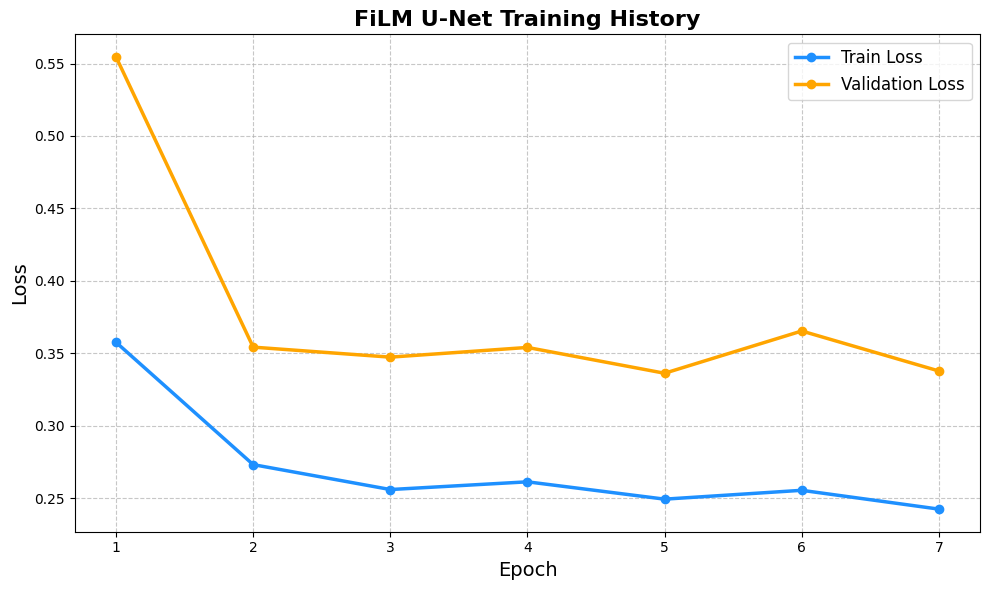
I say begin with above but believe me i already tried a bunch of patching strategies, loss functions, training loops with different hyperparameters, as well as model configs. What I mean is after reaching this level there is still scope to improve model but I didn’t want to do that before investigating and even getting some more data (geographically diverse), which is a process that’s on hold for now.

Evaluation

Evaluating semantic segmentation models on extreme anomalies requires an entirely different methodology than standard classification. If a scene is 99% dry land, a model that simply predicts “dry” everywhere will achieve 99% pixel accuracy. We did try our best to balance the data before training and for validation.

To properly grade this U-Net, I discarded pixel accuracy as a primary metric and built an evaluation suite centered around Intersection over Union (IoU), Precision-Recall (PR), and looked at dynamic thresholding.

Standard binary classification uses a default probability threshold of 0.5. In extreme imbalance scenarios, this is almost always suboptimal. Instead of guessing, I wrote a vectorized threshold search that scans every probability cutoff from 0.01 to 0.99 and calculates the exact F1 score across all pooled validation pixels.

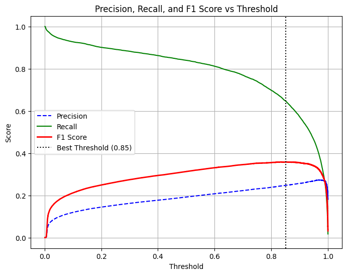
Based on that the best threshold is ~0.85. Because our Focal-Tversky loss was aggressively penalizing False Negatives, the model learned to be highly sensitive, generating a “bloated” probability map. Raising the decision threshold forced the model to be strictly confident before classifying a pixel as water, perfectly balancing precision and recall.

If we look closely at the data, the 0.85 threshold gives a mathematically higher F1 Score (0.58 vs 0.45) and IoU (0.40 vs 0.29) because it pushes Precision way up to 0.75.

But look at what happens to Recall: At 0.85, Recall drops to 0.47. At 0.50, Recall was 0.66

0.85 threshold:
Precision: 0.75
Recall: 0.47
F1-Score: 0.58
Global IoU: 0.4093

0.50 threshold:
Precision: 0.34
Recall: 0.66
F1-Score: 0.45
Global IoU: 0.2910

At 0.85, the model becomes so conservative that it misses 53% of the actual flood pixels (Recall = 0.47). In the real world, failing to predict a flood (False Negative) is catastrophic. Over-predicting a flood (False Positive) is simply an inconvenience.

In flood prediction (and disaster response in general), Recall is king. Missing a flood (False Negative) costs lives and resources; over-predicting a flood (False Positive) just means someone checks a map twice. The mathematical “optimal” threshold of 0.85 choked the model, making it too conservative.

So, for my scenario, I chose to leave the threshold at 0.5, applying this threshold to the unseen Test:

Evaluating U-Net (test)...

--- Global Evaluation Report (GFM_MASK) @ threshold=0.500 ---
              precision    recall  f1-score   support

       False       1.00      1.00      1.00  46551056
        True       0.34      0.66      0.45     33890

    accuracy                           1.00  46584946
   macro avg       0.67      0.83      0.73  46584946
weighted avg       1.00      1.00      1.00  46584946

Global IoU @ threshold: 0.2910
Global pixel accuracy @ threshold: 0.9988

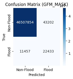
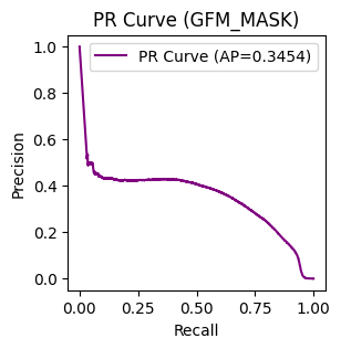
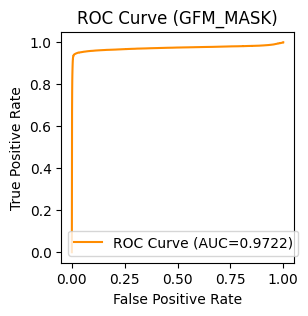
The ROC curve carries the mathematical illusion caused by the 99% dry land in the dataset, the Precision-Recall Curve (middle). This is the bitter truth, the Average Precision (AP) is 0.6558.

Precision is calculated as TP / (TP + False Positives).

Notice what is missing from that equation? True Negatives. The PR curve completely strips away the safety net of the dry land pixels. It forces the model to be judged only on the pixels it flagged as water. It shows that as you try to capture more of the flood (increasing Recall), your model starts making mistakes (dropping Precision).

Above we calculates pixel wise stats, but how does the model do scene wise:

When we break the metrics down scene-by-scene, a glaring geographical disparity emerges. The model achieved a very respectable 0.64 F1 score on the Gatineau scene, but completely collapsed with a 0.17 F1 in Ottawa. Why? Ottawa is a dense urban center. Radar imagery struggles in cities due to “double-bounce” scattering (which makes flooded streets appear bright) and tall building shadows (which mimic the dark voids of deep water). The U-Net and the GFM heuristic labels themselves failed to reliably untangle urban geometry from actual floodwater

Back to our pixel level stats evaluated for patches, while a 99.88% pixel accuracy looks incredible on paper, the Global IoU of 0.29 reveals the model is struggling to perfectly map the micro-boundaries of the water. But metrics only tell you that a model struggled, visuals help you see and analyze better.

To truly evaluate the U-Net, we have to look at the physical predictions overlaid against the raw Sentinel-1 radar and the GFM ground truth.

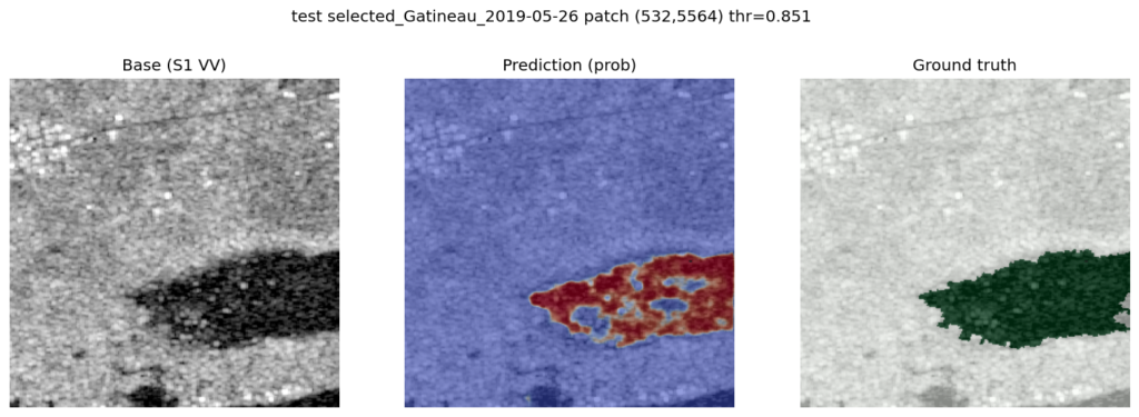
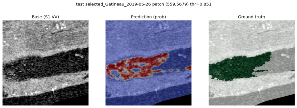
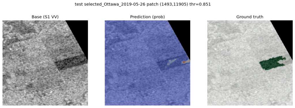
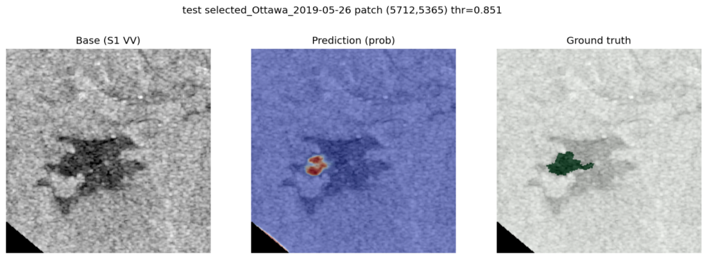
When you look at these overlays, the reality of Earth Observation data becomes clear. The architecture works, but the ground truth is flawed.

1. The U-Net Learned Physics: The model is successfully identifying dark, specular radar reflections (water) and tracking the organic morphology of the river systems. It is finding the physical flood.
2. The GFM Label Noise: The Copernicus Global Flood Monitoring (GFM) targets we trained and evaluated on are not hand-drawn masks; they are generated by heuristic algorithms. If you look closely at the prediction maps, the U-Net is actively predicting flood waters in valid, dark SAR region. Because our evaluation metric treats the GFM mask as absolute “truth,” the model gets heavily penalized (False Positives) for finding water that the heuristic labels ignored

Conclusion

This isn’t the final product but this iteration was promising, so far,

• Built a multi-modal raster pipeline fusing Sentinel-1 SAR with 1D weather vectors and other spatial features
• Implemented an efficient virtual tiling strategy (patches) to dynamically feed a PyTorch DataLoader
• Engineered a FiLM-conditioned U-Net to modulate spatial convolutions based on historical meteorology
• Leveraged a custom Focal-Tversky loss, mixed precision training, and threshold calibration to navigate extreme class imbalance

And the architecture worked. In the context of Earth Observation, extracting an F1 score of up to 0.64 (as seen in the Gatineau scene) on a dataset where the positive class makes up less than 1% of the pixels is a massive signal. It proves that the network successfully bypassed the 99% background noise and learned the actual physical signature of floodwaters.

But the final system boundary we hit wasn’t a failure of code or architecture it was the data taxonomy itself. You cannot train a neural network to achieve perfect physical accuracy using heuristically flawed labels. By forcing the network to optimize against automated GFM data, it wasn’t learning the pure fluid dynamics of a flood; it was just learning to approximate another algorithm’s blind spots.

The U-Net was actively finding floodwaters in valid radar regions, but was mathematically penalized because the automated GFM algorithm had missed them.

Furthermore, the massive disparity between our Gatineau and Ottawa results proved that standard radar approaches inherently struggle with the geometry of dense urban environments.

Clever architectures cannot magically fix fundamental data problems. To map disasters with the precision required for emergency response, the next iteration of this project requires a pivot:

1. Abandoning Heuristic Labels: We need to transition away from automated masks and rely exclusively on hand-annotated, human-validated crisis data (like Sen1Floods11 or Copernicus EMS Rapid Mapping).
2. Exploring Physics-Informed Neural Networks (PINNs): Instead of relying purely on visual pixel segmentation, future iterations should explore embedding the 2D Shallow Water Equations directly into the loss function to force the model to respect the physical laws of fluid dynamics.

Sometimes, the most valuable outcome of a highly engineered ML experiment isn’t a perfect 99% accuracy score (which we already discussed can be quite misleading) it’s proving exactly where, and why, the current data paradigm breaks and where it succeeds.

Though in my humble opinion and the number of iterations it took to get to this iterations, I would say for this data, this score, prediction and accuracy is not bad at all, remember our flood fraction for a scene is << 1% the combination of patching strategies, linear modulation of weather, the water body masks provided as spatial input along with the radar data, the loss function, training loop – all helped significantly.