In the previous posts, we marveled at the elegance of the classical toolkit. We used characteristic equations, matrix exponentials, and integral transforms to perfectly decode the trajectories of physical systems.
But as we established, the classical engine has a fatal flaw: it demands a cooperative universe.
When say an engineer models a spacecraft re entering Earth’s atmosphere, they aren’t dealing with a polite, linear system. They are dealing with hypersonic fluid dynamics, extreme thermal gradients, ablation, and chaotic atmospheric drag. The exact, analytical math shatters under the weight of this nonlinearity.
To survive the real world, we have to step away from the approach of trying to find the perfect equation, or perfect technique that transforms our equation to an easily solvable one, because those methods only get us so far. Instead, we take the data, we discretize reality. We chop time and space into microscopic fragments and allow computers to calculate the future, one tiny frame at a time.
Numerical
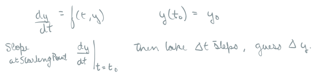
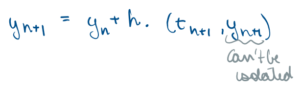
When we cannot find a continuous function y(t) to describe our system, we use time stepping. We take our current, known state, look at the derivative (the slope) at this exact second, and use it to predict where we will be a fraction of a second from now.
Euler
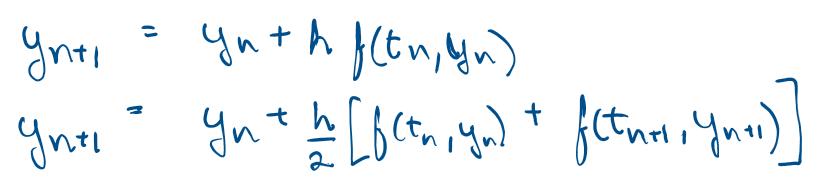
If you know your current position and your current velocity, you simply project that velocity forward over a small, constant time step (h)
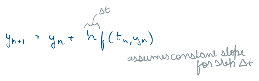
It is a single step approach, explicitly based on the current state. It doesn’t account for history or takes preemptive test steps, the single step approach can be thought of as almost like cutting the Taylor series at 1
For example,
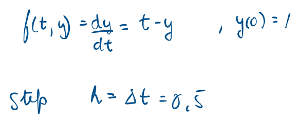
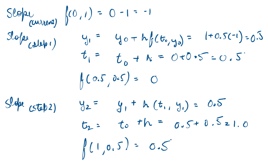
here ‘h’ needs to be microscopic to avoid truncation error under the assumption of constant slope in h timestep
While computationally cheap, Euler’s method is highly inaccurate for chaotic systems. Because it strictly uses the slope at the start of the step, any curvature in the true physics is completely ignored until the next step. Errors accumulate rapidly, causing simulated orbits to artificially decay or spiral out of control.
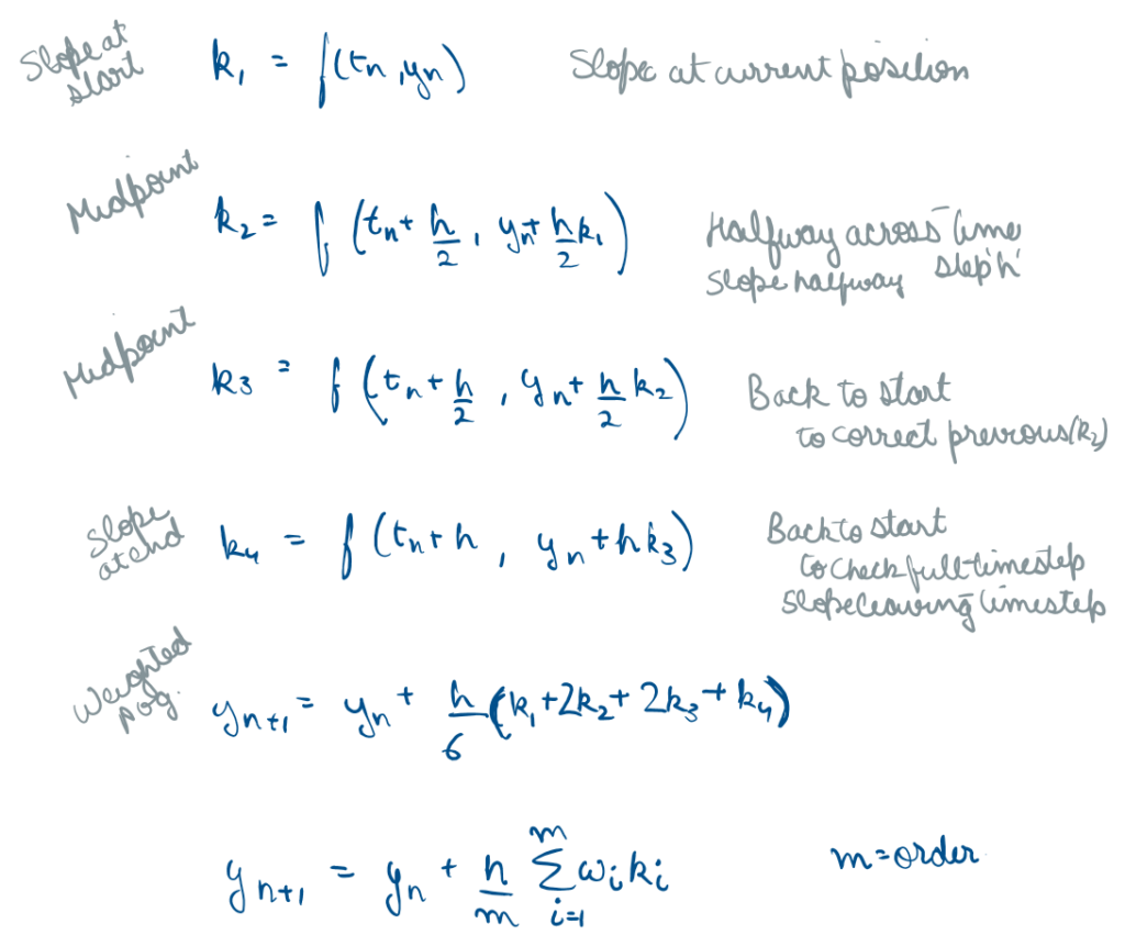
RK – Runge Kutta
Instead of blindly jumping forward based on a single slope, Runge-Kutta methods act like a scout. The standard RK4 method calculates the slope at the beginning of the step, takes a few trial steps to estimate the slope at the midpoint, and checks the slope at the end. It takes a weighted average of these trajectories before committing to the actual step.
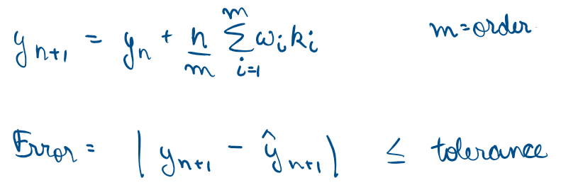
There is RK1, RK2, RK3, RK4 and so on.. where the numeral represents the order, RK4 is the most common (fourth order) – we don’t go any higher as the marginal accuracy doesn’t usually justify the extra compute.
Even though it has the additional power of test steps, its still a single step, explicit and a fixed size step method
In modern physics , we use adaptive solvers like RK45 (DOrmandPrince). RK45 calculates both a 4th order and a 5th order approximation simultaneously. By comparing the difference between the two, the algorithm estimates its own error. If the physical system is currently smooth, it lengthens the time step to save compute power. If the system enters a sharp curve (like a satellite whipping closely around a moon), it dynamically shrinks the time step to maintain high fidelity accuracy.
It features an adaptive time step (varying steps) and acceptable error tolerance, while remaining a single step explicit method.
It helps reduce the chances of incorrect initialization of timestep h in RK4, however it computes 7 slopes at every steps making it a bit compute heavy.
Another alternative is RK23 (Bogacki Shampine), which is a lite version of RK45, using RK2 and RK3, i.e. second and third order approximations, calculating 4 slopes and significantly decreasing compute time (and also accuracy) but it offers a faster alternative in cases where accuracy is not that big of concern.
Heun’s Method
If Euler’s method is walking forward with your eyes closed, Heun’s method is taking a quick peek before you step. It is a two stage process. First, it uses Euler to predict where the system will be. Then, it evaluates the slope at that future prediction and averages it with your current slope to correct the trajectory.
You can either look at it as Predictor and Corrector, where predictor is Euler on current step and corrector is the future step or you can simply look at it as RK2
Adams Bashforth
Runge-Kutta methods are single-step, they throw away all past data and calculate everything from scratch at each new step. But physical systems have momentum. The Adams Bashforth method is a multi-step explicit solver. It looks at the history of your previous slopes to predict the future.
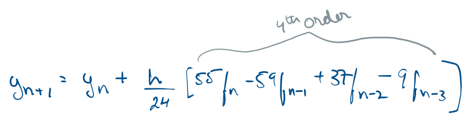
Its fixed multi step explicit process, which accounts for slope at current point n, and previous points n-1, n-2 and so on. Above is an example of a 4th order. It calculates only 1 slope per point and is computationally very fast.
If you are simulating a massive, smooth orbital trajectory, calculating the physics from scratch every millisecond is a waste of compute power. Adams Bashforth recycles the slopes from the last few steps to extrapolate the next one, making it highly efficient for smooth, well-behaved physical systems.
BDF – Backward Differentiation Formulas
Some physical systems are stiff, that is some quantities change way faster than other. This occurs when incredibly fast dynamics and incredibly slow dynamics happen simultaneously – like a rocket’s slow orbital decay paired with the microsecond high frequency vibrations of its thrusters. Explicit solvers (like RK45 or Adams Bashforth) choke on stiffness. They will wildly overshoot the true physics unless you make the time-step microscopically small, which stalls the simulation.
Here we employ a multi step implicit method with adaptive steps. Instead of using the current state to calculate the future, an implicit method sets up an algebraic equation where the future state depends on the derivative of the future state.
In first order, it can be considered as backward Euler. Because the future is trapped inside its own equation, BDF requires us to run a root-finding algorithm (like Newton Raphson) at every single time step just to move forward. It is computationally expensive per step, but it allows us to take massive time steps through stiff physics without the simulation exploding.
So we are essentially using a massive Jacobian to solve for y n+1 at every step
LSODA – Livermore Solver for ODE
Now the question arises, how do we know if a physical simulation is going to be stiff before we hit run? Often, we don’t. A spacecraft’s trajectory might be smooth for three days (non stiff) and then undergo a violent atmospheric re entry (stiff).
LSODA acts like an automatic transmission. It constantly monitors the physics in real time. When the system is smooth, it cruises using the highly efficient Adams Bashforth (explicit) method. The exact millisecond it detects physical stiffness, it drops the clutch and seamlessly shifts into the heavy duty BDF (implicit) mode, preventing the simulation from crashing.
It uses Adams Bashforth, calculates and tracks Lipschitz constant and the changing slope, checks if Adams and h are stable if not resorts to BDF, does periodic checks on stiffness and then resorts back to Adam when needed.
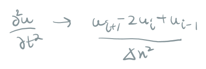
FDM – Finite Difference Method
When modeling the fluid dynamics of an atmosphere or the thermal distribution across a satellite’s solar panel, we must also discretize physical space.
A rigid grid is the oldest and most intuitive way to handle space. FDM shatters the continuous universe into a rigid, rectangular grid of points.
It replaces abstract continuous partial derivatives with discrete algebraic approximations using Taylor series. The derivative at any given point is simply calculated by looking at the difference between its immediate neighbors
the idea is to go from continuous data points -> integer grid
From PDEs -> Algebra
From Algebraic Equation -> Matrix

Under the FDM umbrella, we have two critical schemes for stepping through time:
- FTCS (Forward Time, Central Space): This is the explicit approach. You look at your neighbors right now (Central Space) to predict your exact state in the future (Forward Time). It is incredibly fast to compute, but notoriously fragile. If your time step is even slightly too large compared to your spatial grid, FTCS will violently destabilize.
- BTCS (Backward Time, Central Space): This is the implicit approach. Like BDF, it evaluates the spatial neighbors at the future time step. This forces you to solve a massive system of linear equations simultaneously, but in exchange, it is unconditionally stable. The simulation will never blow up, no matter how large your time step is.
SOR – Successive Over-Relaxation
Systems like BTCS, generate a massive matrix representing thousands of interconnected spatial points, inverting a 1,000,000 x 1,000,000 matrix directly is very expensive, hence, we use iterative methods. We make a wild guess at the entire temperature grid, and then iteratively update each point based on its neighbors.
Now what is ‘over relaxation’ – SOR deliberately overshoots the correction based on a relaxation factor (omega), hence the name.
By mathematically “leaning” into the direction of the correction, SOR dramatically accelerates the convergence, allowing us to solve massive atmospheric or thermal grids in a fraction of the computing time
I haven’t looked into it in too much detail yet but i’d recommend going through – https://primer-computational-mathematics.github.io/book/c_mathematics/numerical_methods/6_Solving_PDEs_SOR.html
FEM – Finite Element Method
In FDM, we discretize a continuous space into rigid rectangular grid, but that doesn’t work for all situations where our space is possibly curved or asymmetical. FEM instead is based on geometry, it instead decomposes the space into geometric elements – a flexible mesh – could be triangles, tetrahedron, line segments
Then it uses integration by parts to convert the differential equation into an integral over volume problem, this process is called weak formulation, where instead of trying to satisfy the differential equation exactly at every point, it multiplies the physics by “test functions” and integrates across the area of each triangle. By assembling these thousands of tiny local integrals into one massive global matrix, FEM perfectly captures complex, real-world geometries that FDM could never handle.
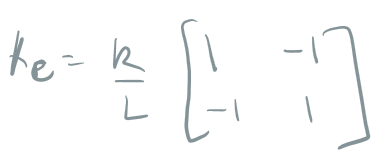
Then it assumes basic shape functions (e.g. Linear Interpolation for line segments geometry) say N1 and N2
Then calculates integrals using the basic shape functions above to create a Local stiffness matrix (Ke)
Then it combines the local matrices to a global one
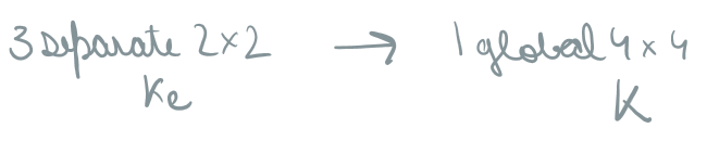
and then applies the boundary condition
Conclusion: The Computational Bottleneck
In the real world, the universe does not hand us neat, analytically solvable equations. To model the chaotic realities of aerodynamic drag, orbital decay, or atmospheric thermodynamics, we have to discretize reality.
By stepping carefully through time with algorithms like RK45 and LSODA, and by shattering continuous space into grids and meshes using FDM and FEM, we have successfully taught computers how to simulate the physical universe. These traditional numerical methods are the undisputed workhorses of modern engineering. They are the software engines that currently guide our satellites and predict our weather.
But they have a fatal flaw: they are incredibly computationally expensive.
When you scale these methods up to simulate the fluid dynamics of an entire planet or the real time aerodynamics of a rocket launch, the matrices become so massive that even supercomputers choke. Sometimes, simulating a complex weather system using traditional numerical grids takes longer than the actual weather takes to arrive.
We have reached the limits of pure, brute force computation. To push the boundaries of Earth Observation and astrophysics forward, we cannot just keep building finer grids and taking smaller time steps. We need a fundamental paradigm shift.
We need to stop forcing computers to calculate physics from scratch, and start teaching them the laws of physics.
In Part V: Scientific Machine Learning, we will cross the final frontier. We will explore how to merge the raw predictive speed of Artificial Intelligence with the absolute deterministic rigor of classical calculus, resulting in the architecture that is actively reshaping research in the field: Physics Informed Neural Networks (PINNs).
References
On Runge-Kutta processes of high order – Cambridge University press
Leave a Reply