In last part, we learned how to solve isolated differential equations, a single pendulum swinging, a single spring oscillating. But physical reality is rarely isolated, and it is rarely smooth.

What happens when a physical system experiences a violent, instantaneous shock, like a sudden thruster burn on a satellite? The continuous, well behaved polynomials we’ve relied on shatter. Furthermore, what happens when variables are inextricably linked? The pitch, roll, and yaw of a spacecraft tumbling in orbit cannot be solved one at a time, they are a coupled system of equations where every movement bleeds into the next.

To survive this level of complexity, we have to change our mathematical perspective a bit.

Analytical – Integrals

When the time domain becomes too chaotic to navigate, we don’t force our way through it. Instead, we use integral transforms to teleport the entire differential equation into a different mathematical dimension, solve it there using basic algebra, and then teleport the solution back.

Fourier

Imagine taking a chaotic, noisy signal plotted on a standard x-y graph (amplitude over time). The Fourier Transform takes that time based wire and physically wraps it around a circle. The speed at which you wrap the wire around the circle is the frequency (omega)

• If your winding frequency omega does not match any frequency hidden inside the signal, the peaks and valleys cancel each other out. The wire winds symmetrically, and the center of mass stays perfectly dead-centered at the origin (0,0)
• But, if your winding frequency exactly matches a hidden frequency embedded in the noise, the peaks align. The wire bulges heavily to one side, and the center of mass spikes away from the origin.

The Fourier Transform is simply a mathematical radar sweeping through every possible winding frequency. When the center of mass spikes, you have detected a pure wave hidden inside the chaos.

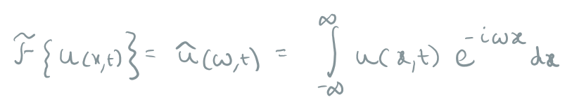
Mathematically, the engine that drives this circular winding is the complex exponential e^(-i*omega*t)
By multiplying our time domain signal by this winding engine and integrating across all of time, we calculate that center of mass and hence convert the math from the time domain (t) into the frequency domain (omega)

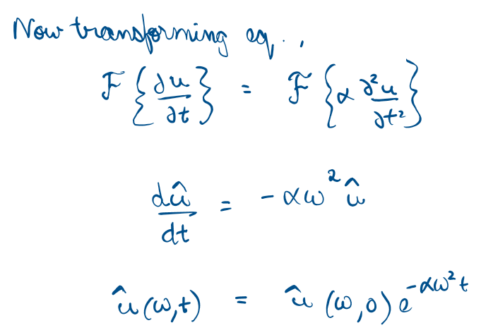
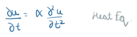
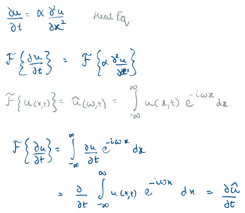
Because in the frequency domain, the complex derivatives of a Partial Differential Equation (like that of the Heat Equation or wave equations) collapse. By decomposing our physical reality into a pure spectrum of simple sine and cosine waves, we can solve the math for each individual frequency using basic algebra, and then add them all back together.

Once again, here is an excellent visualization of how this works by 3Blue1Brown:

But what is a Fourier series?  From heat flow to drawing with circles | DE4

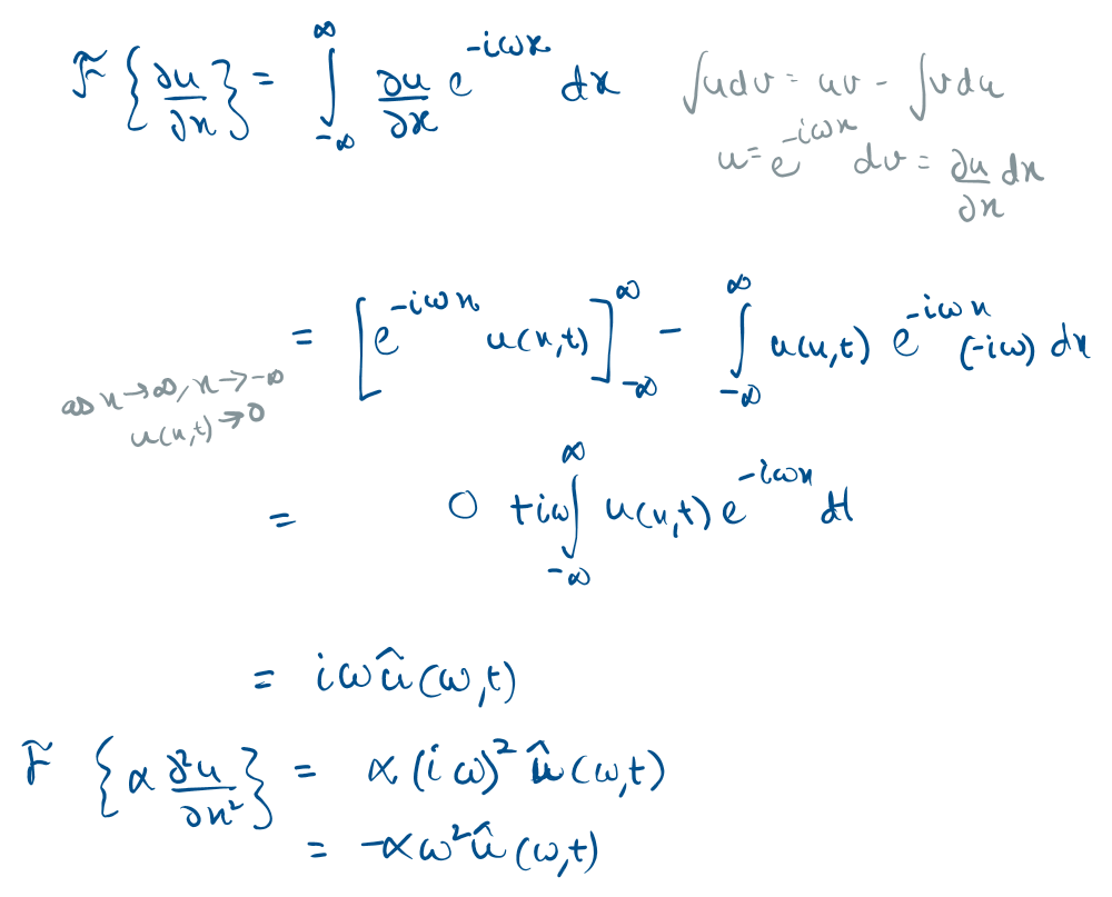
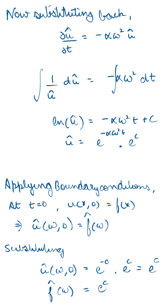
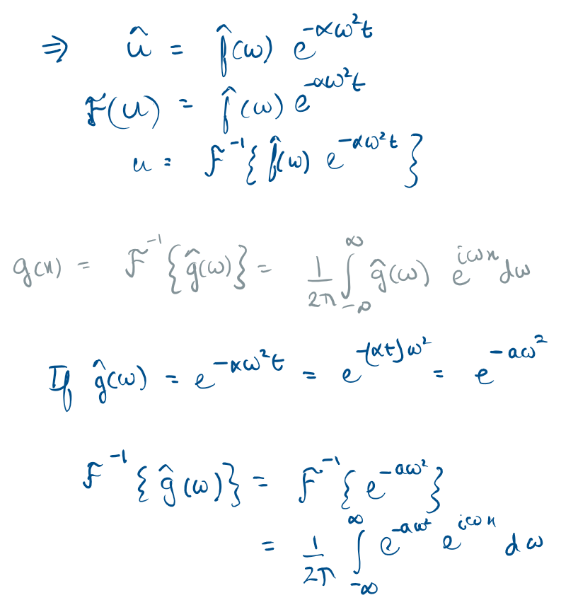
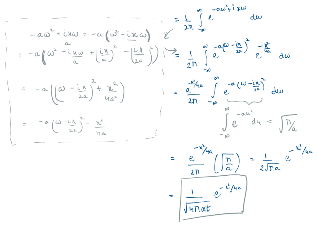
Following is the solution of heat equation using Fourier transforms:

Laplace

Laplace also helps us to transform our equation from a time domain (t) to a frequency domain (s).

Imagine a satellite silently coasting through the vacuum of space. Suddenly, a micrometeorite strikes its hull, or an onboard computer fires a 0.5-second thruster burst to correct its orbit. In the time domain (t), these events are mathematical nightmares.

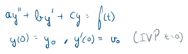
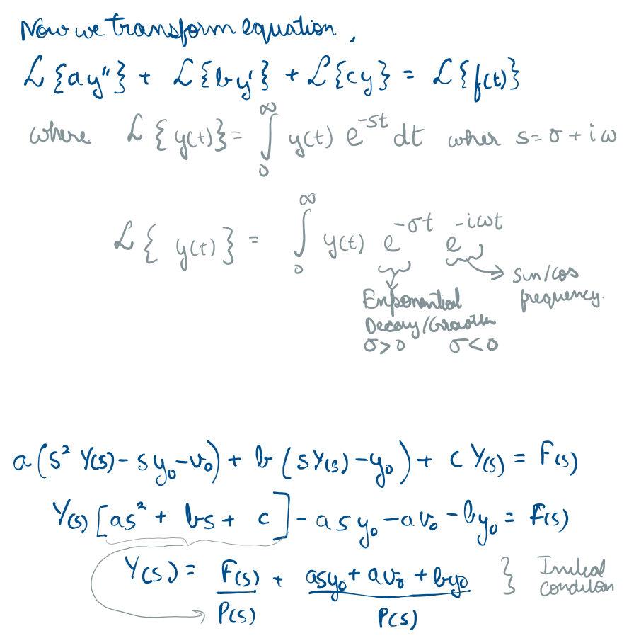
By integrating the differential equation alongside a decaying exponential e^(-st), the Laplace transform converts complex derivatives into simple algebraic multiplication.

The following video by 3 blue 1 brown gives an excellent visual intuition of what it does, how it does it and how it really works, definitely check it out :

But what is a Laplace Transform?

How it works is:

Instead of tracking when things happen, the s-domain (s = sigma + i*omega) tracks the anatomy of the system’s behavior specifically, its exponential decay and sinusoidal frequencies.

Unlike Fourier which just winds the signal around a circle, Laplace introduces a modifier – a real number exponential decay factor (e^-sigma*t i.e. geometrically – a spiraling, shrinking vortex) and hence it takes the exploding signal and forcibly squashes it down so that it shrinks as time goes forward and Only after the signal has been safely squashed does the machine wind it around the circle

Because s is made of two dimensions (the squashing factor sigma on the x axis, and the winding frequency omega on the y axis), the output of the Laplace Transform isn’t a simple 2D graph but a 3D topographical map over the complex plane, on which we look for Poles i.e. points where the map shoots up into infinitely high spikes.

• The y axis (omega) tells you how fast the system naturally oscillates or vibrates.
• The x axis (sigma) tells you the system’s survival. If a pole lands on the left side of the map (negative sigma), the system naturally decays and stabilizes. If a pole lands on the right side of the map (positive sigma), the system grows exponentially and will physically destroy itself.

There is another video by 3 blue 1 brown summarizing these applications way better:

Why Laplace transforms are so useful

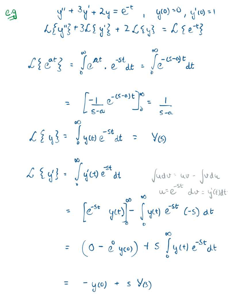
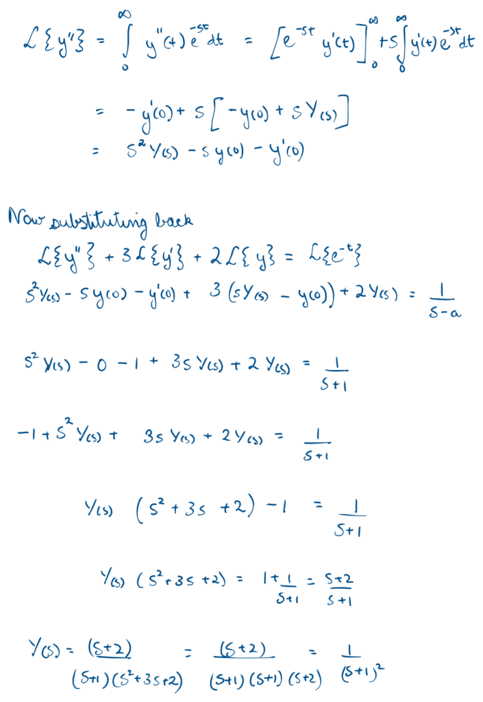
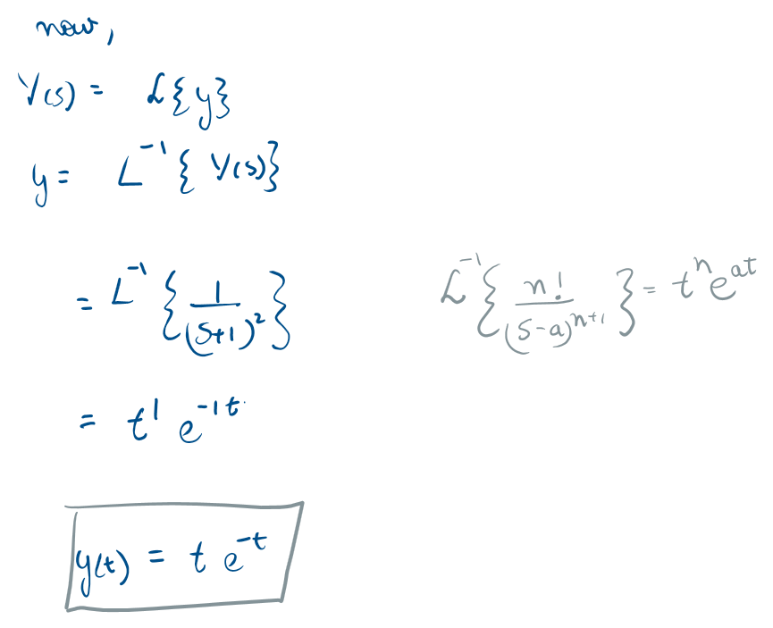
Here is an example of how this method can be applied to solve equations:

Analytical – Systems

In classical physics, we often model systems as if they exist in a vacuum, focusing on a single variable changing over time. But reality is entangled.

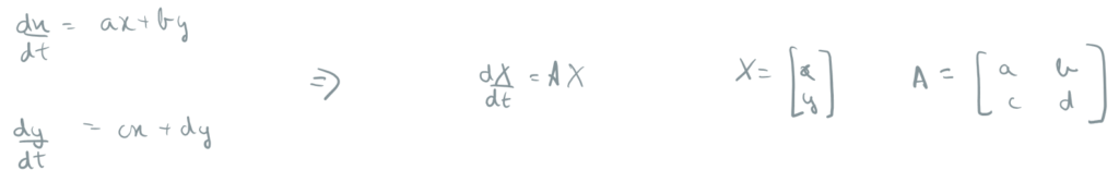
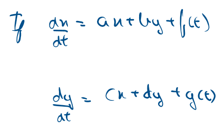
When you model the orbital dynamics of a multi-body system, or the pitch, roll, and yaw of a satellite, the rate of change of one variable depends directly on the current state of all the others. We are no longer dealing with a single equation, we are dealing with a matrix of differential equations:

Substitution

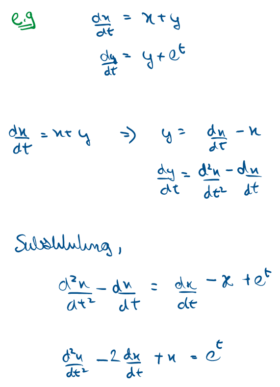
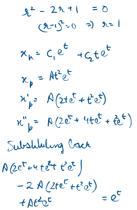
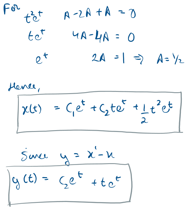
If we have a simple system of two coupled variables, say, the coupled velocities of two masses on a vibrating string, the most classical approach is simply to eliminate one of them to see the whole picture

By isolating one variable in the first equation and substituting its derivative into the second, we can crush a system of two first order ODEs into a single, uncoupled second order ODE. We then solve this using the classical characteristic equations we learned in Part II. It works perfectly for simple systems. But as you add a third, fourth, or fiftieth dimension, this brute force algebraic substitution collapses under its own weight.

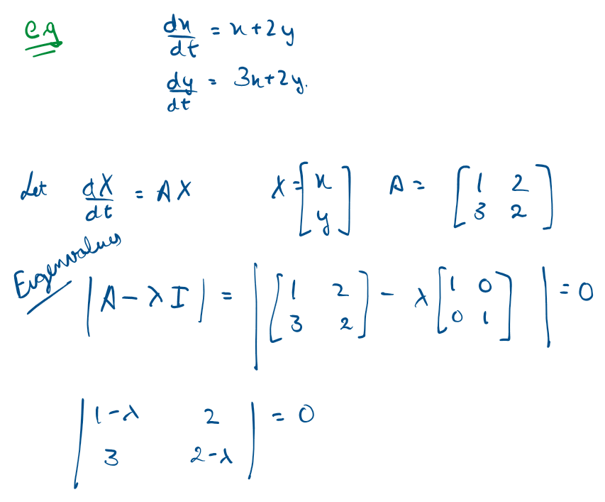
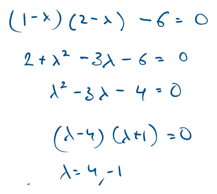
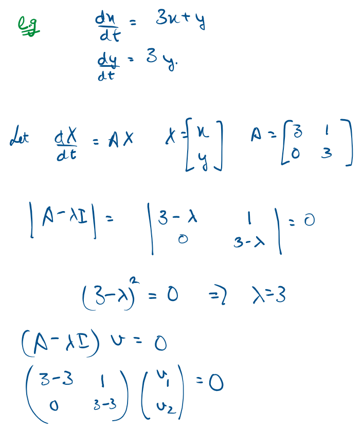
Eigen Value & Eigen Vector

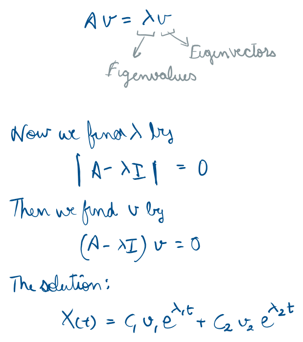
Let’s go back to our satellite tumbling out of control in orbit. From the outside, the chaotic mixture of pitch, roll, and yaw looks incredibly complex to model. But if you shift your perspective to look down the exact right angles, the principal axes of rotation, the motion suddenly makes perfect sense. The satellite is just spinning cleanly around these invisible lines.

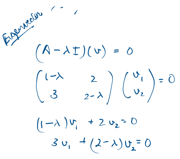
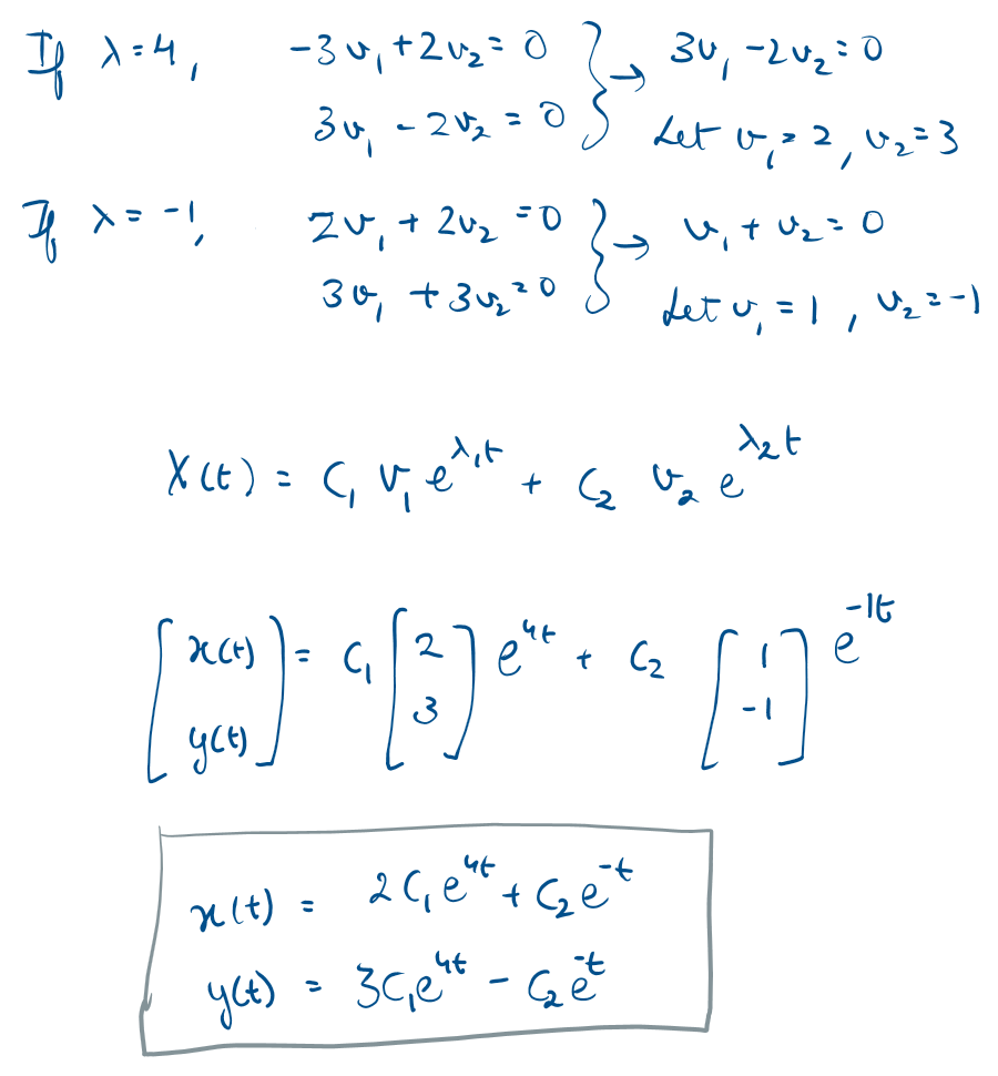
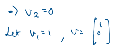
This is exactly what Eigenvectors (v) and Eigenvalues (lambda) do for our system of differential equations. The Eigenvectors act as those fundamental axes. They represent the specific directions in our multidimensional space where the coupled system behaves as if it were completely uncoupled. The corresponding Eigenvalues dictate exactly what is happening along that specific axis, whether the motion decaying, growing, or oscillating.

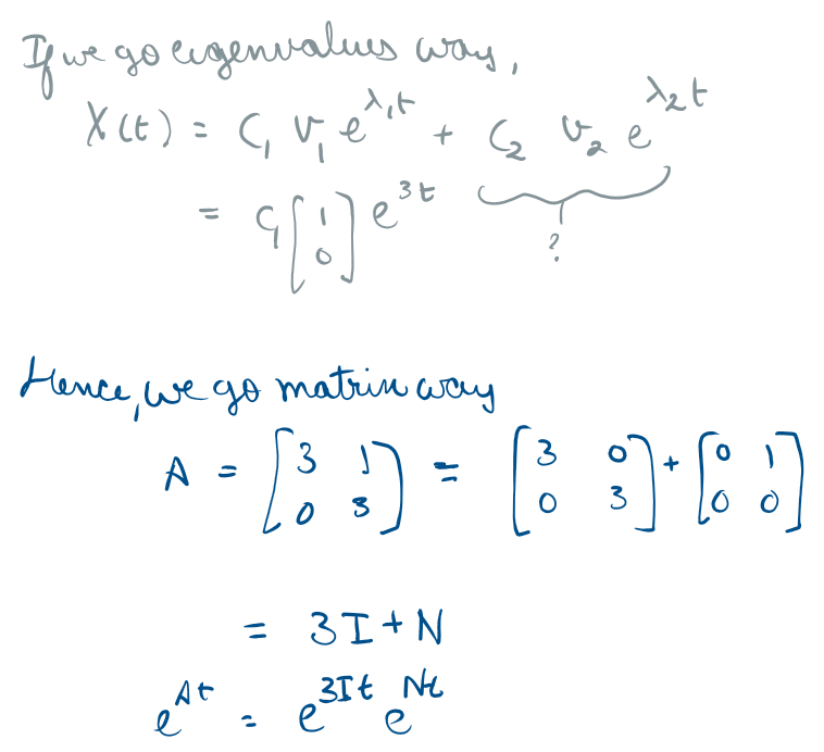
By breaking the equation into eigenvalues and eigenvectors, we end up converting our equation into independent solvable threads of exponential growth and decay

Matrix Exponential

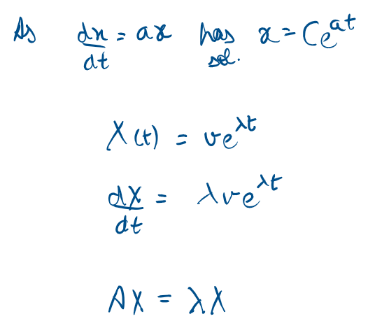
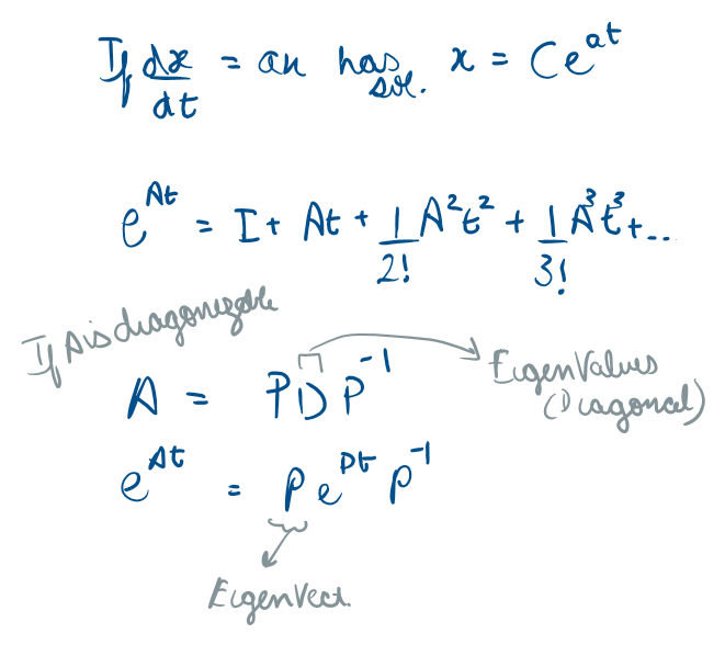
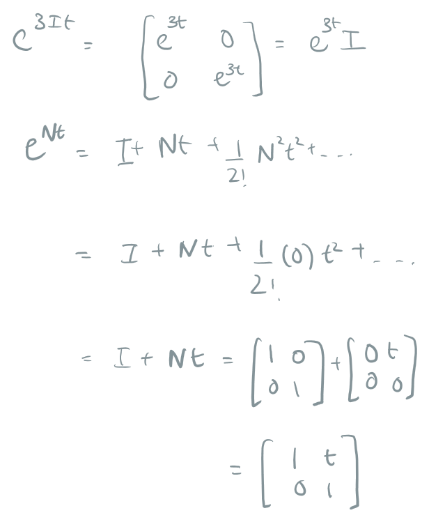
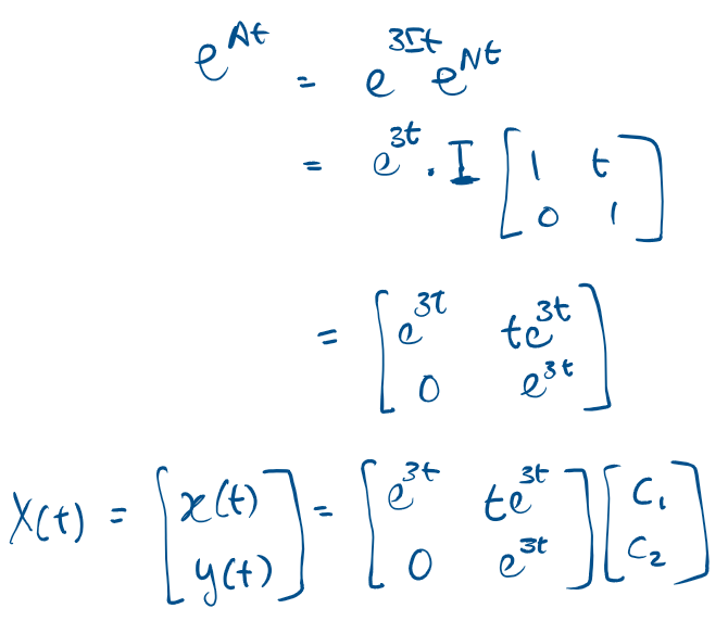
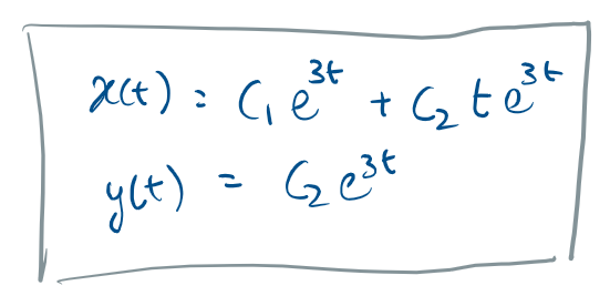
In Part I, we learned that the fundamental blueprint for a 1D linear differential equation (x’ = ax) is the exponential function: x(t) = C e^(at). But what if a isn’t a single number? What if A is a massive matrix containing the physical constraints of an entire spacecraft.

We can still use the same math, but challenge here is how to interpret e raised to an entire matrix,
we use the infinite Taylor series expansion, or we use our Eigenvectors to diagonalize the matrix

Another 3Blue1Brown video explaining this beautifully:

How (and why) to raise e to the power of a matrix | DE6

Conclusion

With integral transforms and state-space mechanics, we have reached the absolute peak of the exact mathematical world, for the most part at least. We have learned how to untangle massive matrices of coupled variables which could potentially predict a spacecraft’s orientation, and we have learned how to map explosive, discontinuous physical shocks into clean, algebraic frequency domains.

These analytical tools are monumental achievements. They are the mathematical engines that put humanity on the moon and allow us to filter the noise of the cosmos.

All of the elegant methods we have discussed, from characteristic equations and matrix exponentials to Laplace and Fourier transforms, rely heavily on the assumption that the underlying physical system is linear, or at least polite enough to be approximated as such.

But the real universe is rarely polite.

When we introduce extreme nonlinear chaos, like the unyielding fluid dynamics of atmospheric entry, the unpredictable N-body gravitational tug-of-war, or the massive spatiotemporal datasets of modern Earth Observation, our exact equations shatter. The matrices become too large, the integrals become unsolvable, and the classical math breaks down.

To survive the bleeding edge of modern physics and engineering, we hand the geometry over to the machines.

In Part IV, we will explore the Numerical Methods that actually run inside modern mission control simulators, culminating with the Physics-Informed Neural Networks (PINNs)

References

But what is a Fourier series?  From heat flow to drawing with circles | DE4

But what is a Laplace Transform?

Laplace in Spherical Coordinates

Why Laplace transforms are so useful

How (and why) to raise e to the power of a matrix | DE6