In Part I, we explored the geometric blueprints of differential equations. We looked at first order systems and how we can occasionally use clever substitutions to bypass the curse of nonlinearity.

But the physical universe is rarely satisfied with first order changes. Gravity, electromagnetism, and orbital mechanics all rely on acceleration – the rate at which the rate of change is changing. To model these, we need second order (and possibly higher) differential equations.

When the universe hands us a linear, higher order system, we don’t have to guess blindly. We have a pristine, toolkit designed to tear these equations apart and solve them analytically. Let’s look at some of these methods.

Analytical – Higher Order

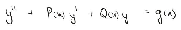
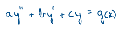
When we deal with linear higher-order ODEs, we divide our physical reality into two states: Homogeneous (unforced systems operating in a vacuum g(x) = 0) and Non-Homogeneous (systems being pushed or pulled by an external force, g(x) != 0)

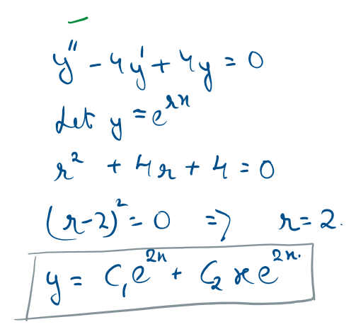
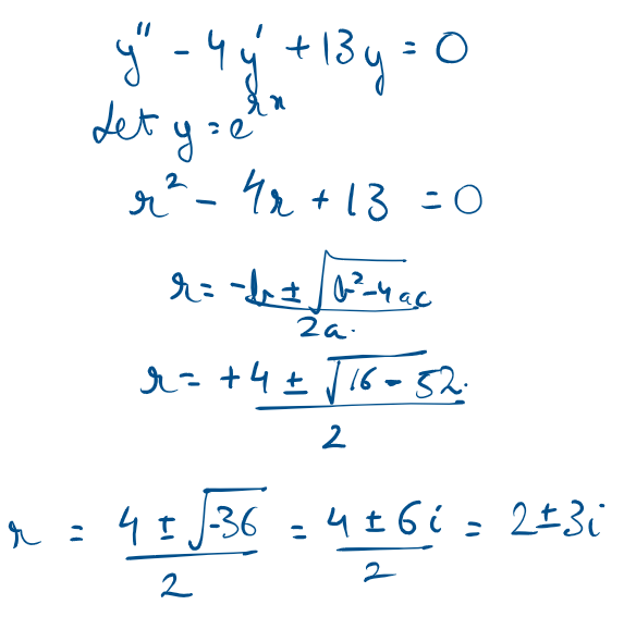
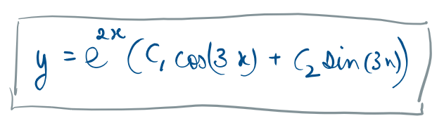
Characteristic Equation

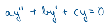
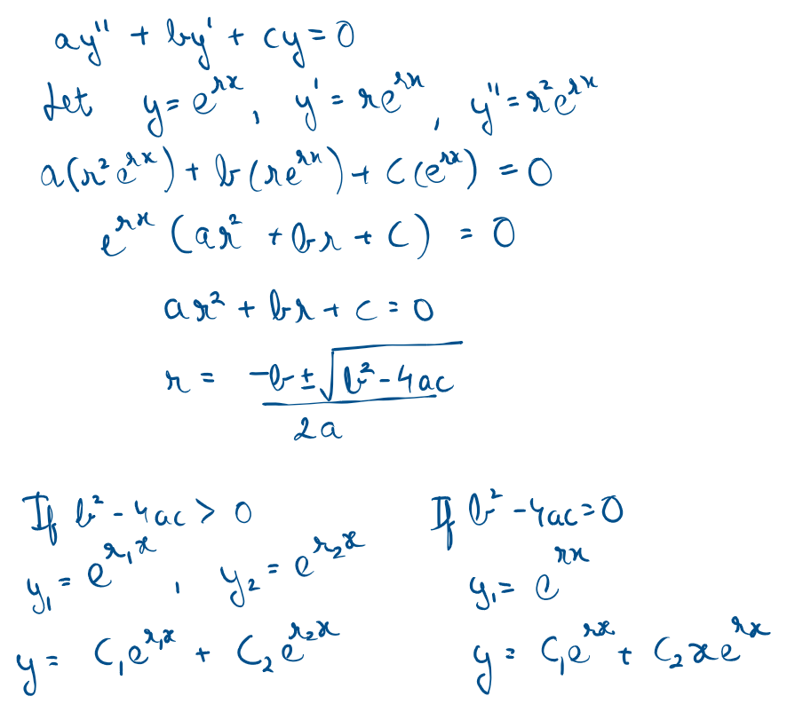
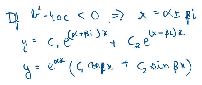
Its a simple straightforward strategy for solving higher order homogenous equations (systems with no external forces acting on it) with constant coefficients (P(x) and Q(x) are constants). The intuition is to substitute an exponential such that the equation can be solved like a simple quadratic equation.

The physical intuition is to solve an equation where a function, its velocity, and its acceleration all balance out to zero, we use a function that is completely immune to calculus,

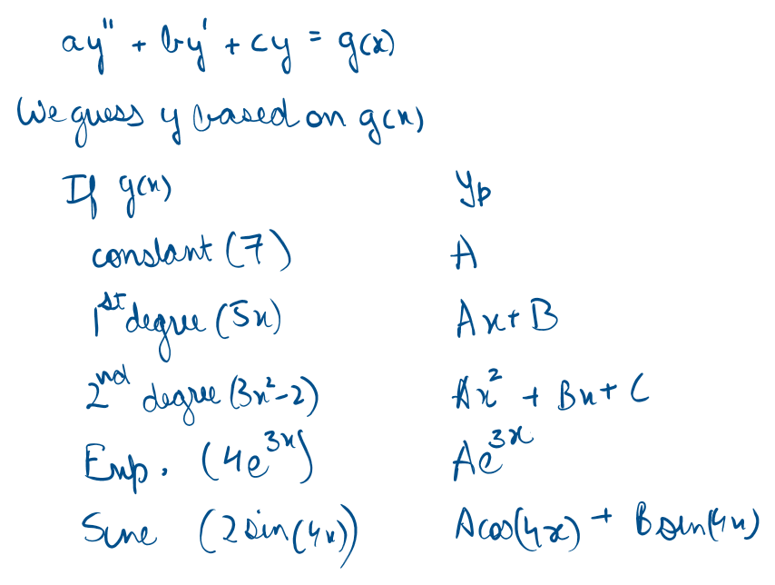
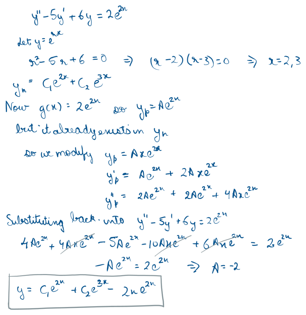
Method of Undetermined Coefficients

Now lets move to the case of constant coefficients but a non homogenous situation (i.e. g(x) != 0)

This strategy relies on the assumption that a system will eventually mimic the force acting upon it, If the forcing function g(x) is relatively simple (a polynomial, an exponential, or a sinusoid), we simply guess that our final solution will have that exact same shape, plug it into the ODE, and solve for the missing coefficients.

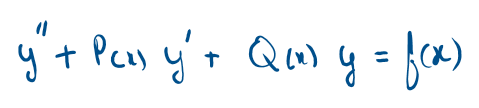
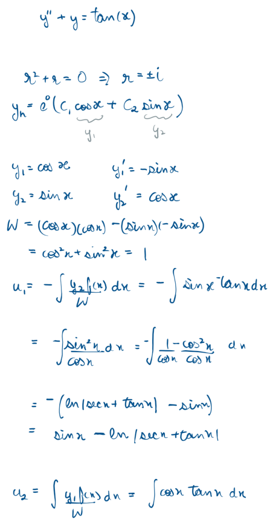
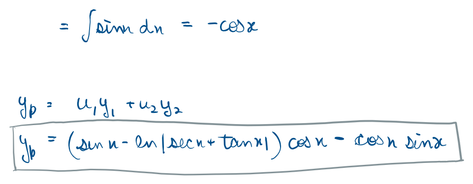
Variation of Parameters

Now we move onto the case where our function is not a simple one that we can guess a solution to, i.e. f(x) here isn’t a simple function.

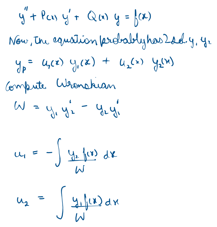
This is a bit more complicated than the previous ones, what we do here is, instead of guessing a rigid shape, we take the constants (C1, C2) from our homogeneous solution and allow them to “breathe”. We transform them into evolving functions of time: u1(x) and u2(x). By using a mathematical construct called the Wronskian (which checks the fundamental independence of our solutions), we can integrate these parameters to find the exact trajectory of the system, no matter how weird the forcing function is

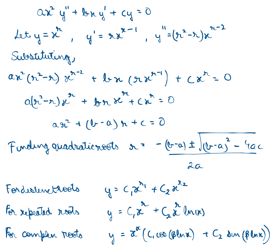
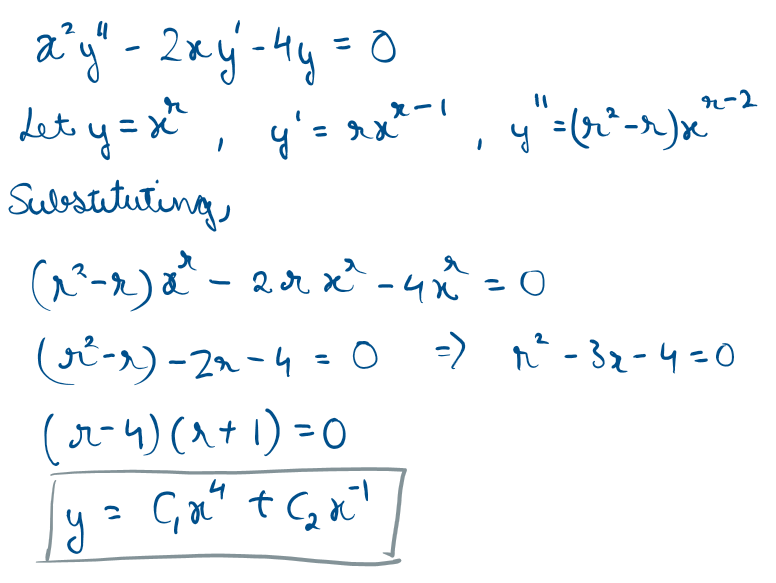
Cauchy Euler

The cases we discussed so far involved only constant coefficients, now we move to equations where P(x) and Q(x) aren’t necessarily constant.

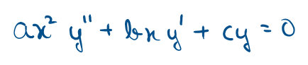
These kind of equations can model spherical or cylindrical symmetry, like calculating the gravitational potential deep inside the layers of a star, or the heat distribution expanding across a circular radar dish.

Because the power of the x coefficient exactly matches the order of the derivative here, our trusty exponential guess doesn’t work, so instead we guess a polynomial, and substitute to transform the equation into a solvable algebraic equation.

Analytical – Series

What happens when the coefficients are not constants, the symmetry is broken, and the universe hands us a completely unsolvable mathematical mess?

We stop trying to find a neat, closed form equation. Instead, we build the solution from scratch, piece by piece, using infinite series

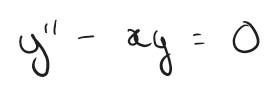
In this case for instance if we let y = e^rx or y = x^r, the x acting as a coefficient of y creates a problem.

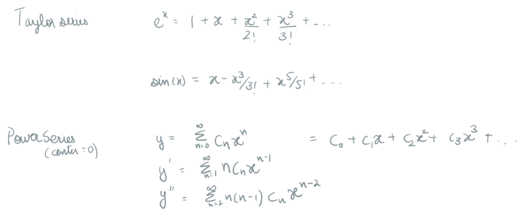
Hence we leverage infinite series like Taylor series and the Power series to build up the solution

Ordinary Points

This method is applicable only to systems with analytic function as the coefficients (i.e. P(x) and Q(x) are smooth and defined at 0)

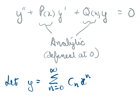
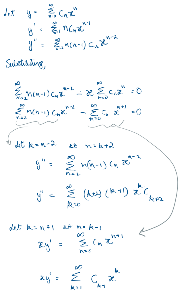
Because the space is smooth, we assume our solution can be perfectly described by an infinite Power Series, We differentiate this infinite sum, plug it back into our ugly differential equation,

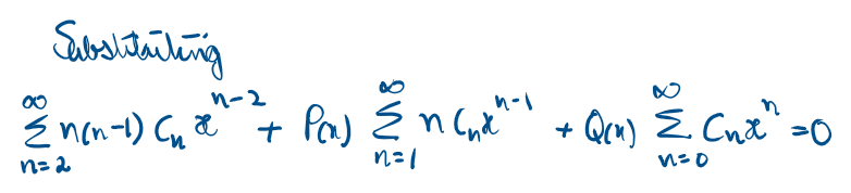
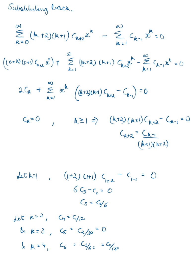
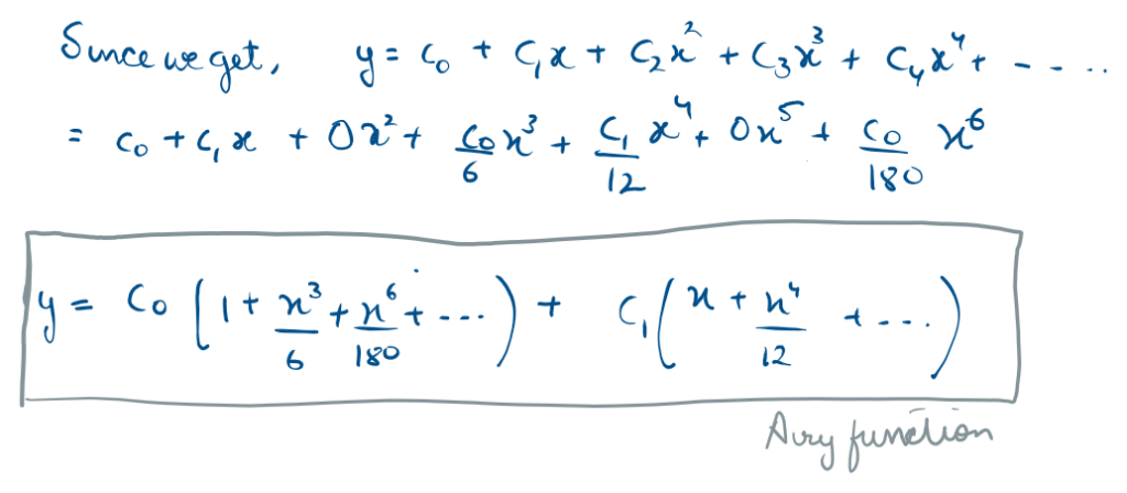
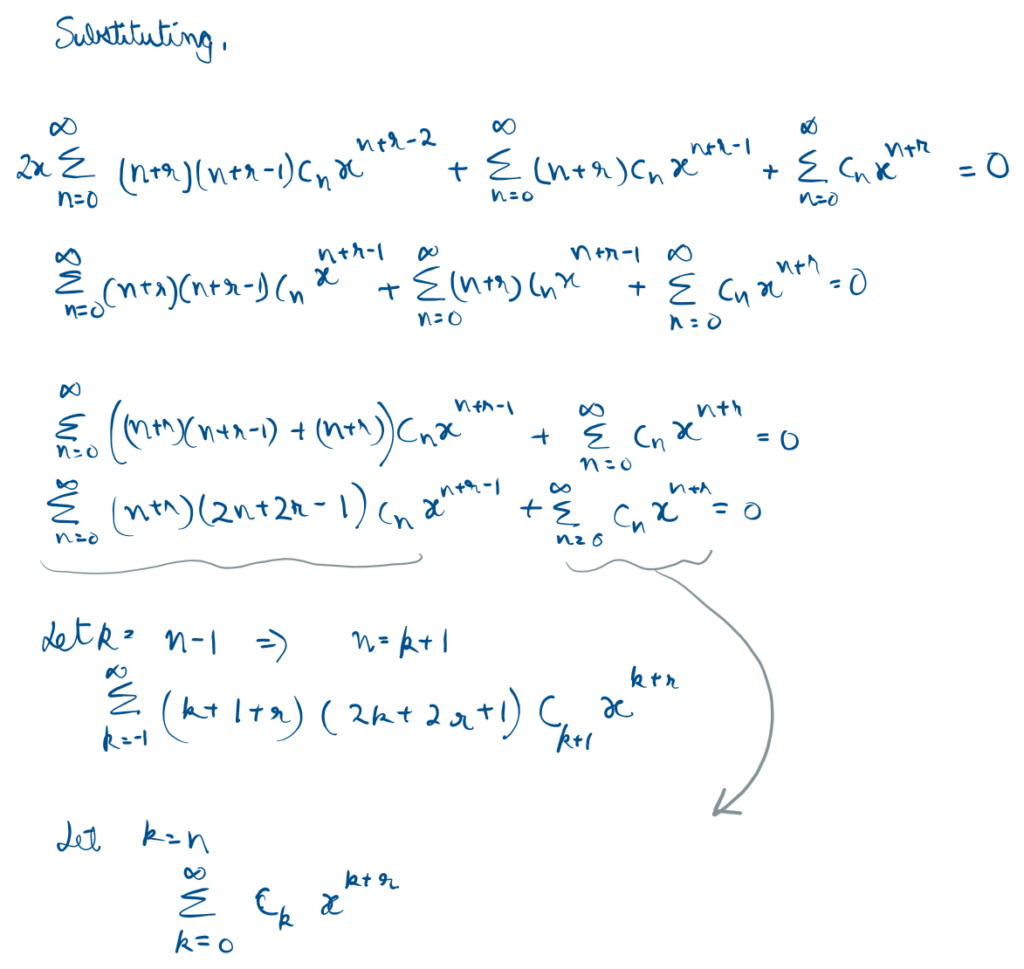
To solve this, we shift the indices until all the powers of x align. This gives us a “recurrence relation” a master algorithm that computes every single coefficient (c0, c1, c2..) one by one, building the true physical curve with as much precision as we have the patience to calculate

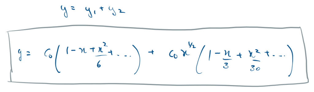
Frobenius

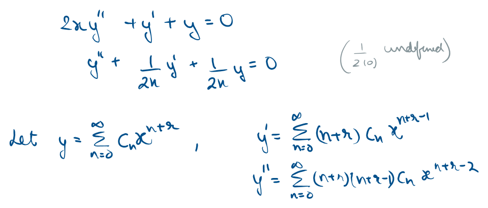
This method is applicable to systems with non analytic function as the coefficients (i.e. P(x) and Q(x) are not defined at 0)

Imagine calculating the electric field exactly at the center of a point charge, or modeling the physics at the event horizon of a black hole. At these locations, the physical variables blow up to infinity. In differential equations, this mathematical tear in the fabric is called a Singular Point

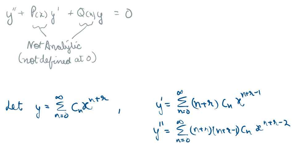
We modify our infinite series by multiplying the entire thing by an extra parameter of x^r

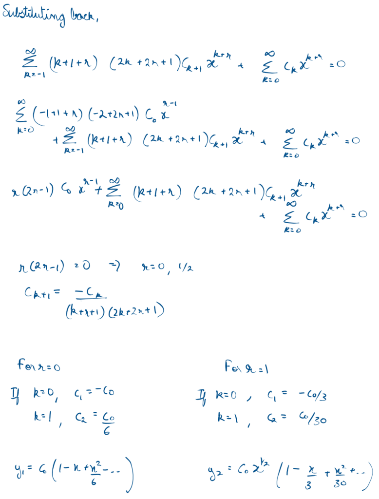
By finding the roots of the “indicial equation,” we adapt the geometry of our math to navigate around the singularity, allowing us to find valid physical solutions even when the universe tries to break the rules

Conclusion: The Limits

Classical analytical methods and infinite series are monumental achievements of human intellect. They allow us to peer into the mechanics of the universe, decoding the exact trajectories of pendulums, the vibrations of satellite antennas, and the intense physics warping around singular points.

But as powerful as this classical engine is, it has its limits.

What happens when a physical system experiences a violent, instantaneous shock, like a sudden thruster burn on a spacecraft, or a lightning strike on a power grid? The continuous, smooth geometry we’ve relied on shatters. Polynomials and infinite series struggle to describe sudden, violent discontinuities.

Furthermore, series solutions are fundamentally local. They build reality step-by-step from a single starting point, but they don’t easily give us a global view of a massive, multi-variable system.

To handle the true chaos of modern engineering and astrophysics, we have to entirely change our mathematical perspective. We have to stop looking at time and space directly, and instead transform our equations into the domains of frequency and complex variables. And when even those advanced analytical tools fail us against the crushing weight of nonlinearity, we have to teach machines to solve the physics for us.

In Part III, we will cross that final frontier. We will explore Integral Transforms (Laplace and Fourier) and finally, the Numerical Methods and Physics Informed Neural Networks (PINNs) that power modern computational research.