What is a Loss Function?
As an intuitive understanding loss would be predicted value – actual value i.e. how much off is prediction to our actual target, most of you might be familiar with R^2 loss in high school which is what we often compute while fitting points to a line.
Loss function is what quantifies the discrepancy between what the model thinks reality is, and what reality actually is.
For a single training example i.e. a single data point, it outputs a scalar representing that specific prediction’s error. When we average this error across an entire dataset or a mini batch during optimization, it becomes the Cost Function or Objective Function that the model tries to minimize.
Now why are Loss function important in ML?
Just like a physical system works on the principle of Least action (Lagrangian)
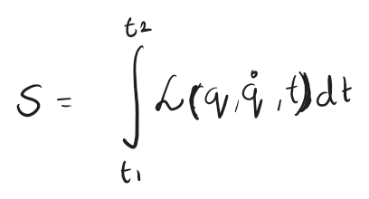
What it means is, nature basically evaluates the Lagrangian (difference of kinetic energy and potential energy) – and defines the path of the particle – which is the path of least action.
That is how our ML models also learn – following the path of least action i.e. decreasing loss function – to get to a better and better understanding of the inherent relations in the data to either output those or to output a prediction.
There are a ton of loss functions out there – some of the most common ones like RMSE, MAE, MSE etc. for regression like problems and CE, BCE, Log Loss, Hinge Loss etc. for classification like problems, we will probably cover those in detail some other time and you could try to get familiar with the basics here if you want:
https://www.datacamp.com/tutorial/loss-function-in-machine-learning
In this post I will cover some loss functions I’ve been using in my current iteration on a project involving imbalanced classification on an image (pixel level classification).
Pointwise
Pointwise functions would be those, that take into account single prediction and true value, compute loss and decide how much it should weigh in overall fitting / learning trajectory.
Binary Cross Entropy (BCE)
The essence of this function lies in framing the problem as a series of independent coin flips, what that means is – we calculate the loss (log loss actually) of each pixel independently.
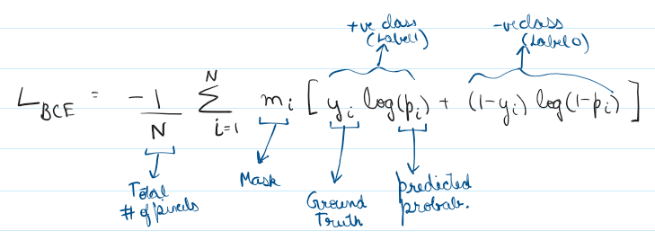
Which if you think about it, will heavily penalize confidently incorrect predictions (using a log scale!)
Walkthrough
Now to demonstrate how it works, lets work with this example:
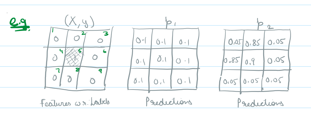
We have this image with 9 pixels in which only 1/9 is flooded (our target class)
Now our first model generates a series of predictions p1, which completely misses our target, which is common in a binary classification if a class imbalance isn’t handled properly, what it means is, if the model trains on data thats 99% dry (target 0) – classifying all pixels as class 0 is a guaranteed way to optimize accuracy.
in this example, our loss would come out to be:
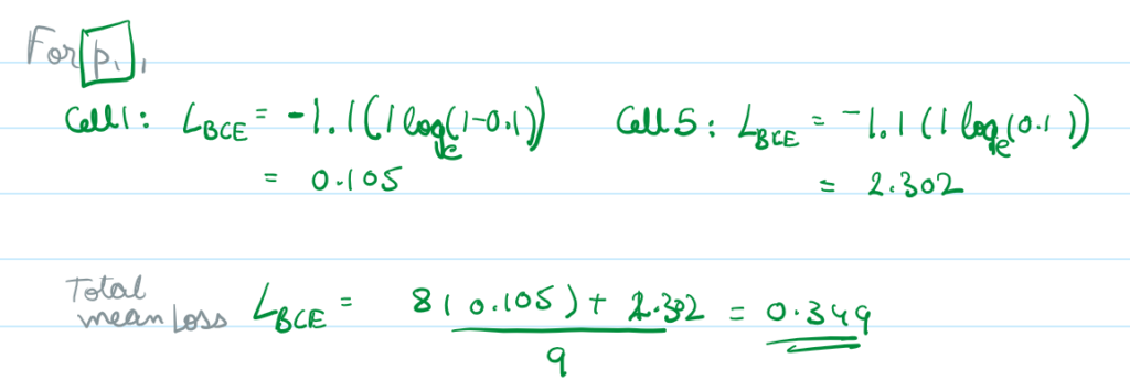
Now lets look at p2, the predictions of another model (or second iteration of this one), the model correctly classifies the flooded pixel and in a way localizes the neighborhood as well, i.e. some pixels next to the flooded pixel also get classified as flooded, in this case:
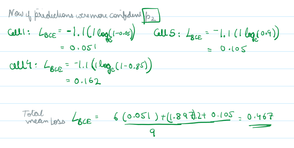
So if we evaluate these two iterations with BCE we would assume that p1 is superior to p2
Notes
- Measures distance between predicted and true probability distributions
- Best for balanced binary classification problems
- It is a convex function – smooth gradient
- Probabilistic – so helps callibrate for max likelihood
- could have runtime errors with log(0) -> -inf
- Pytorch implementation han ln and also has BCEWithLogitsLoss (Sigmoid + BCE) implementation
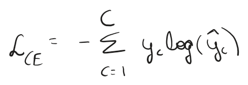
Cross Entropy
Cross entropy is for multi class mutually exclusive labels
| Feature | Binary Cross-Entropy (BCE) | Cross-Entropy (CE) |
| Number of Classes | C = 2 | C > 2 |
| Output Activation | Sigmoid | Softmax |
| Output Layer Shape | 1 neuron (or N independent) | C neurons (one per class) |
| Class Relationship | Independent (Can have multiple true labels) | Mutually Exclusive (Only one true label) |
| Target Label Format | Scalars (0 or 1) or multi-hot vectors | One-hot encoded vectors (or probability distribution) |
| Gradient Interaction | Gradients for each node are calculated independently. | Gradients are coupled across all output nodes via Softmax. |
Focal
Focal Loss was an improved, dynamically modified BCE, that was introduced by Facebook originally for a R-CNN framework.
The essence of this function is that unlike BCE that treats all errors equally, Focal loss introduces weights, and down weights the well classified examples forcing the network to mine for hard examples.
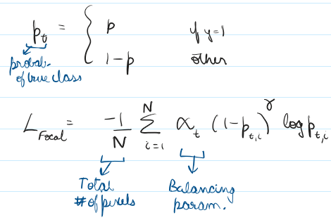
It has two hyperparameters alpha and gamma, gamma term makes for the modulating factor dictating how much should samples who are easily classified weigh and alpha helps tune loss function to the inherent imbalance of the dataset.
Intuition is that,
- gamma controls the steepness of the penalty for being wrong
- alpha roughly reflects the inverse frequency of classes, but must be dampened if using a high gamma
Usually we start with gamma = 2.0 and alpha = 0.25 (which roughly corresponds to the true target being 25% of the values)
Walkthrough
Now to demonstrate how it works, lets work the same example as above:
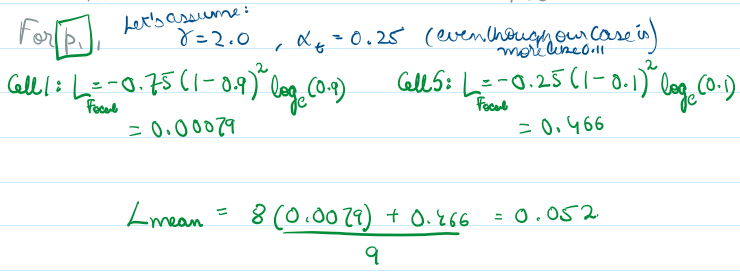
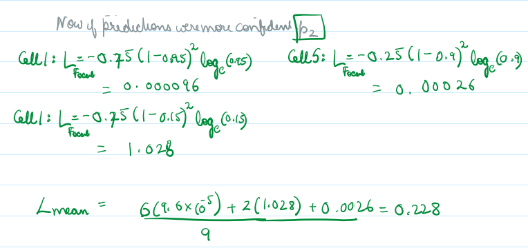
Here we see if a pixel is classified easily, like p = 0.95 (i.e. for the void pixels of prediction 0.05), the modulating factor with gamma, reduces their contribution to overall loss function significantly.
Notes
- A good potential solution for highly imbalanced datasets (especially the highly sparse ones)
- Makes network focus on its representational capacity
- Mines for rare / hard samples
- Potentially very sensitive to noise – minor noise could be treated as extremely rare samples and dictate the optimization direction
- Computationally its significantly more expensive than BCE
- Numerical stability needs handling when p approaches 0 or 1
- Performance highly dependent on hyperparameter selection (alpha and gamma) – adds another layer of tuning/selection
Overall – Macro Boundaries
Instead of pixel level attribution, these evaluate overall overlaps and use the True Positives, False Negatives, false Positives etc. in their calculations, letting you optimize for the desired outcome directly.
These are called geometric or boundary functions because they focus on preserving the decision boundary.
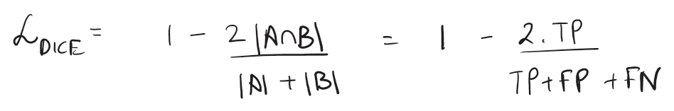
Dice
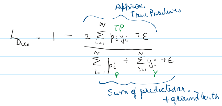
It is used to calculate overlap between predicted mask and ground truth, or as we call Intersection Over Union (IoU). The essence is the function ignores the background altogether and cares only about true and predicted values of target class.
Walkthrough
To explain how this works, we will consider this example:
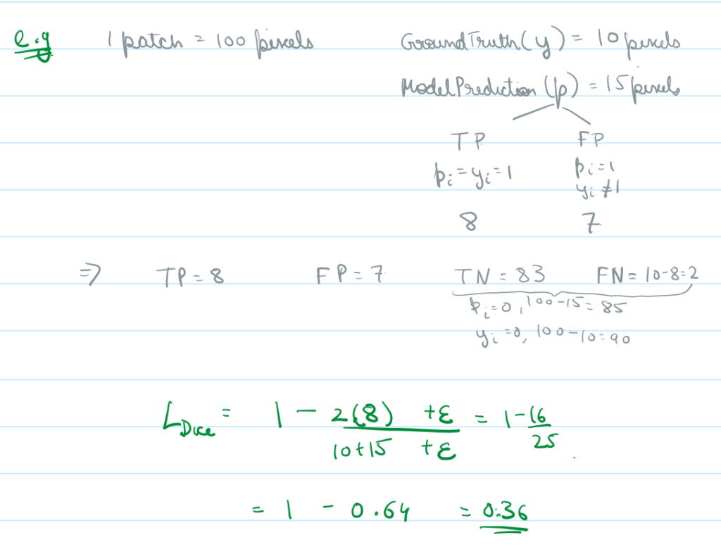
Here we have an image of 100 pixels, in which 10 are flooded (i.e. our target class) and the rest 90 are class 0.
Now, lets say our model predicts 15 of the 100 pixels to be flooded, in which only 8 are truly flooded (True Positives).
This means we have 7 false alarms (False Positives), and we missed 2 true floods (False Negatives) and the rest 83 were non flooded which we guessed correctly (True Negatives)
As you can see even though TN make about 83% of our data – we don’t really care for them in our loss function.
Notes
- Blind to TN
- It directly optimizes for IoU which is the metric we care about
- Its good when preserving boundaries is important (Medical Imaging / SAR)
- Its inherently balanced since intersections are relative
- because of the mentioned scale invariance – can swing wildly from image to image i.e. missing 100 pixels in 10k pixels is a way smaller penalty than missing all 10 in 10
- By itself – its a non convex function and would be challenging to find a global minima – causing unstable gradients
- Its blind to the types of errors – our use case cares about FP more than FN or vice versa – this loss function does not accommodate that calibration
- Needs the term epsilon added – to prevent division by 0 during runtime (prone to vanishing gradients)
Tversky
Basically modified Dice with two parameters alpha and beta added to tune the FP and FN weight as per use case requirement. Th idea is that not all mistakes carry same penalty.
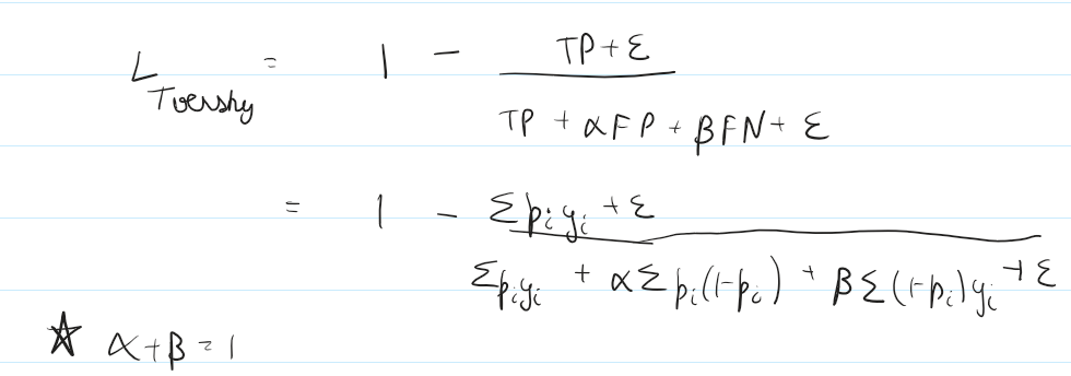
alpha = beta = 0.5 => we have dice loss function
alpha < beta => Penalizing FN (Optimizing Recall) – Missing a true label is more expensive
alpha > beta => Penalizing FP (Optimizing Precision) – Being confident in true labels is critical
Walkthrough
To explain how this works, we will consider the same example:
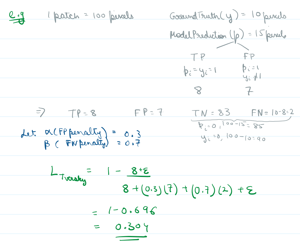
Here we have an image of 100 pixels, in which 10 are flooded (i.e. our target class) and the rest 90 are class 0.
Now, lets say our model predicts 15 of the 100 pixels to be flooded, in which only 8 are truly flooded (True Positives).
This means we have 7 false alarms (False Positives), and we missed 2 true floods (False Negatives) and the rest 83 were non flooded which we guessed correctly (True Negatives)
Now, if the model instead made the opposite error (2 False Positives and 7 False Negatives), the denominator would become 8 + (0.3 * 2) + (0.7 * 7) = 13.5, resulting in a Tversky Index of 0.59 and a higher Loss of 0.41. The math explicitly punishes the network harder for missing the target than for over predicting it
Notes
- pretty much same as dice, completely blind to true negatives
- great for real world usecases / risks – lets optimize penalties for FP, FN
- Like focal loss – sensitive to parameter selection – adds another layer of hyperparameter tuning and selection
- Because of hyperparameter weighting – can be really sensitive to noise – if say FN penalized highly i.e. beta = 0.9, model would overindex and bloat target label predictions
- Can optimize better for Recall than Dice
- like dice non convex – can lead to unstable gradients if used by itself
- Same issues as Dice for scale invariance – can fluctuate wildly from image to image
- Same issues as Dice needs the term epsilon added – to prevent division by 0 during runtime (prone to vanishing gradients)
Conclusion
There are a number of widely tested loss functions which are better suited to a specific problem and model, I would recommend trying with the most basic ones for the first prototype and then researching the ones best suited to your use case, you might need to define a custom one yourself too! But I hope this post helps give some insight into few of the ones covered, I’ll follow up with a deep into some other ones.
Implementation
In my case I’ve tried to implement a combination of pointwise and overall loss functions
Focal + Tversky:
class FocalTverskyLoss(nn.Module):

  def __init__(
    self,
    focal_alpha: float = 0.25,      # focal class weight on positive pixels
    focal_gamma: float = 2.0,      # down-weight easy pixels: (1 - pt)^gamma
    tversky_alpha: float = 0.3,    # FP cost in Tversky denominator
    tversky_beta: float = 0.7,     # FN cost (β > α → recall-friendly)
    smooth: float = 1e-5,          # epsilon - to prevent division by 0
    tversky_weight: float = 1.0,
  ):
    super().__init__()
    # focal loss
    # alpha indicates class weight to positive class, gamma is the modulating factor
    self.focal_alpha, self.focal_gamma = focal_alpha, focal_gamma
    # tversky loss
    # beta = 0.8, alpha = 0.2  - penalizes FN 4x times more than FP
    self.tversky_alpha, self.tversky_beta = tversky_alpha, tversky_beta
    # smooth - epsilon - to prevent division by 0
    self.smooth, self.tversky_weight = smooth, tversky_weight

  def forward(self, logits, targets, valid_mask=None):
    #extract valid area to ignore void pixels
    m = torch.ones_like(targets) if valid_mask is None else valid_mask.float()
    #total number of pixels (valid)
    n = m.sum() + self.smooth

    # --- Focal: batch-level pos_weight in BCE, then (1-pt)^gamma focusing ---
    # with torch.no_grad():
      # TP count
      # pos = (targets * m).sum()
      # TN count
      # neg = ((1 - targets) * m).sum()
      # dynamic ratio of positive to negative  (capped at 50)
      # pos_w = (neg / (pos + self.smooth)).clamp(1.0, 50.0)  # rare-flood upweight
    # calculate BCE
    # bce = F.binary_cross_entropy_with_logits(logits, targets, reduction="none", pos_weight=pos_w)
    bce_unweighted = F.binary_cross_entropy_with_logits(logits, targets, reduction="none")
    pt = torch.exp(-bce_unweighted)
    # static alpha balancing map
    alpha_t = self.focal_alpha * targets + (1.0 - self.focal_alpha) * (1.0 - targets)
    # Focal formula
    # focal = (w * (1 - pt).pow(self.focal_gamma) * bce_unweighted * m).sum() / n
    focal_map = alpha_t * (1.0 - pt).pow(self.focal_gamma) * bce_unweighted
    focal = (focal_map * m).sum() / n

    # --- Tversky: soft tp/fp/fn per sample, then mean(1 - index) ---
    # Converts raw logits to probabilities and zeroes out invalid pixels
    p = (torch.sigmoid(logits) * m).flatten(1)
    # Flatten Ground Truth
    t = (targets * m).flatten(1)
    tp = (p * t).sum(1)
    fp = (p * (1 - t)).sum(1)
    fn = ((1 - p) * t).sum(1)
    # Tversky Formula
    tversky = 1 - (tp + self.smooth) / (tp + self.tversky_alpha * fp + self.tversky_beta * fn + self.smooth)
    # Averages the Tversky scores across the batch and adds the Focal loss
return focal + self.tversky_weight * tversky.mean()BCE + DICE loss (assuming its for more or less balanced datasets):
class BCEDiceLoss(nn.Module):
    def __init__(self, smooth: float = 1e-5):
        super().__init__()
        self.smooth = smooth
        self.bce = nn.BCEWithLogitsLoss(reduction="none")

    def forward(self, logits: torch.Tensor, targets: torch.Tensor, valid_mask: torch.Tensor = None) -> torch.Tensor:

        if valid_mask is None:
            valid_mask = torch.ones_like(targets)

        valid_mask = valid_mask.float()

        # BCE Loss (masked)
        bce_map = self.bce(logits, targets)
        bce_loss = (bce_map * valid_mask).sum() / (valid_mask.sum() + self.smooth)

        # Vectorized Dice Loss
        probs = torch.sigmoid(logits)

        # Flatten spatial dimensions to [Batch, Features]
        batch_size = probs.shape[0]
        p_flat = (probs * valid_mask).view(batch_size, -1)
        t_flat = (targets * valid_mask).view(batch_size, -1)

        inter = (p_flat * t_flat).sum(dim=1)
        p_sum = p_flat.sum(dim=1)
        t_sum = t_flat.sum(dim=1)

        dice_score = (2.0 * inter + self.smooth) / (p_sum + t_sum + self.smooth)
        dice_loss = (1.0 - dice_score).mean()

return bce_loss + dice_lossResources
Basic intuition
- https://www.datacamp.com/tutorial/loss-function-in-machine-learning
- https://www.kaggle.com/code/nghihuynh/understanding-loss-functions-for-classification
Relatively Comprehensive Landscape
Focal Loss: