“Change is the only constant in life”

That’s also how the universe works in a way and how we study it, how something changes with respect to another and differential equations is what we use to describe this.

The universe is not a static photograph it is a continuously evolving engine. Whether we are modeling the orbital decay of a satellite, the fluid dynamics of a hurricane, or the heat dissipating across a spacecraft’s hull, we are studying how one physical state changes with respect to another. We use them to model almost physical behavior from pendulums and projectiles, celestial objects, air resistance and heat equation.

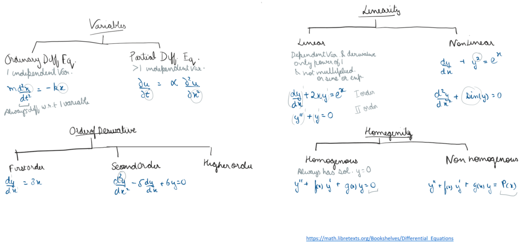
Now going into the terminologies and symbolism of these equation, we broadly categorize differential equations into two types

Types – The Anatomy of Change

If the changes are with respect to a single variable for example change in 1D, 2D or even 3D space with respect to time, we call these Ordinary Differential Equations (ODEs)

Imagine tracking the trajectory of a satellite in Low Earth Orbit (LEO). Its position and velocity change as time marches forward. The equation simply asks: Given your exact coordinates and momentum right now, where will you be in the next instant? It traces a single, deterministic thread through space.

If the system is governed by multiple inputs like temperature change in a rod that changes with both distance and time, we formulate them as Partial Differential Equations (PDEs)

The temperature depends not just on when you measure it, but exactly where on the 3D surface you measure it. You are no longer tracking a single thread; you are modeling the entire fabric of the system.

Phase Space & Stability Analysis: Seeing the Future

In the real world, finding a clean, exact mathematical solution is rare. Before we even attempt to calculate a specific answer, we look at the geometry of the equation to determine the overall stability of the system. We do this by mapping the equation into a Phase Plane.

In a phase plane, we don’t plot position against time. We plot the state variables against each other, for example, position (x) on one axis and momentum (v) on the other.

When you map a differential equation into phase space, it generates a vector field. This field acts like a fluid flow of arrows, dictating the exact destiny of the system. By analyzing this geometry, we can identify critical equilibrium points:

1. Attractors (Stable): If a satellite is in a perfectly stable, repeating orbit, the phase space vector field will show all nearby arrows spiraling inward toward a closed loop or a single point. No matter where the system starts nearby, it will be pulled into this stable configuration.
2. Repellers & Saddle Points (Unstable): If a satellite is experiencing atmospheric drag and its orbit is decaying, the vector field reveals an unstable geometry. Even a microscopic perturbation a slight change in solar wind or atmospheric density will cause the trajectories to diverge wildly, pushing the system into chaos or forcing the satellite to burn up in the atmosphere.

Stability analysis allows us to understand the fate of a physical system simply by looking at the geometry of its derivatives, without ever solving the equation.

The following 3 blue 1brown video has a very nice visualization of phase space towards the end of the video, of how these phase spaces look like for some of the popular and even completely arbitrary differential equations

Differential equations, a tourist’s guide | DE1

Now you must be asking, i geometric intuition is so powerful, why do we need dense analytical methods or massive computational solvers?

The answer lies in the difference between linear and nonlinear realities.

When a differential equation is linear, its vector field is neat, predictable, and symmetrical. It obeys the principle of superposition, you can break the system into smaller, manageable pieces, solve them individually, and seamlessly add them back together.

But the universe is rarely that accommodating.

When systems become nonlinear, the geometry becomes entangled. The vector fields twist, fold, and exhibit extreme sensitivity to initial conditions. For a long time, this was a mathematical dead end.

However, we don’t always have to immediately surrender to heavy computers. For certain, highly specific first-order nonlinear systems, mathematicians have discovered brilliant analytical loopholes. These analytical techniques act as mathematical sleight of hand. They even allow us to temporarily warp the geometry of a nonlinear equation, disguising it as a linear one just long enough to solve it cleanly by hand. (We will explore these exact analytical tricks in the next section).

The true “curse” of nonlinearity only reveals itself when systems scale up.

When we move beyond isolated first-order equations into massive, coupled nonlinear systems, like the N-body problem governing the gravitational tug-of-war between satellites and moons, or the Navier-Stokes equations dictating disaster-scale weather patterns, our analytical intuitions only get us so far. To survive in that chaotic geometry, we are forced to abandon exact human calculations and approximate reality using heavy numerical solvers and even Physics-Informed Machine Learning. (We will explore these computational architectures in later posts.

Solving Differential Equations

There are several ways we can solve a differential equation, there are a couple of Analytical as well as Numerical methods, lets first discuss analytical ways we can solve these equations, it can be as simple as solving a linear equation or can be a Laplacian or involve integrating by parts, the way to solve depends on the type of differential equations.

Analytical Methods – First Order

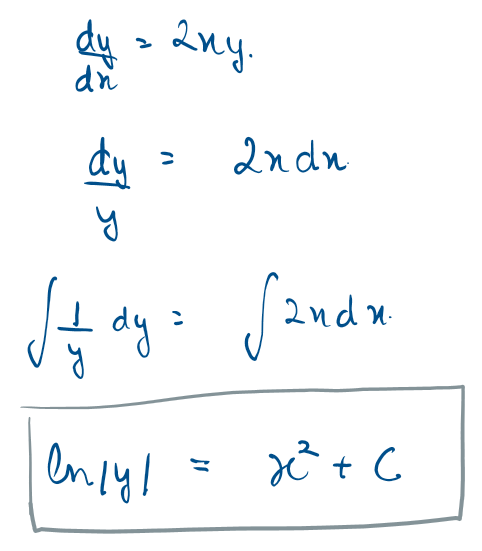
Separation Of Variables

Probably the simplest most intuitive way to solve differential equations, a number of differential equations – both ODEs and PDEs of first order

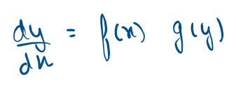
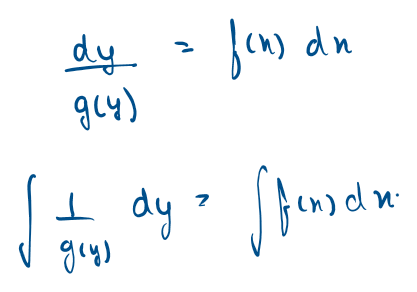
The intuition is to separate the two variables and integrate separately.
Imagine trying to untangle two different colored strings that have been tightly knotted together. Separation of variables is the mathematical equivalent of pulling the red string to the left and the blue string to the right until the knot dissolves. The intuition is that if the physical forces acting on a system are independent of each other, their mathematics should be independent too

This is so vital in physics and you must have used this while solving for heat equation or exponential decay separating temporal and spatial changes and integrating them 1 by 1

The only limitation of this simplistic strategy is – it only works when the function is not very complex and is easily separable – but as you’ll see that’s not always the case.

Working through an example

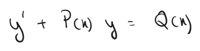
Integrating Factor

A universal approach to solving first order linear equations

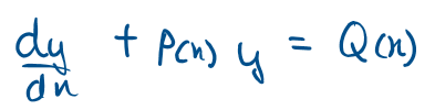
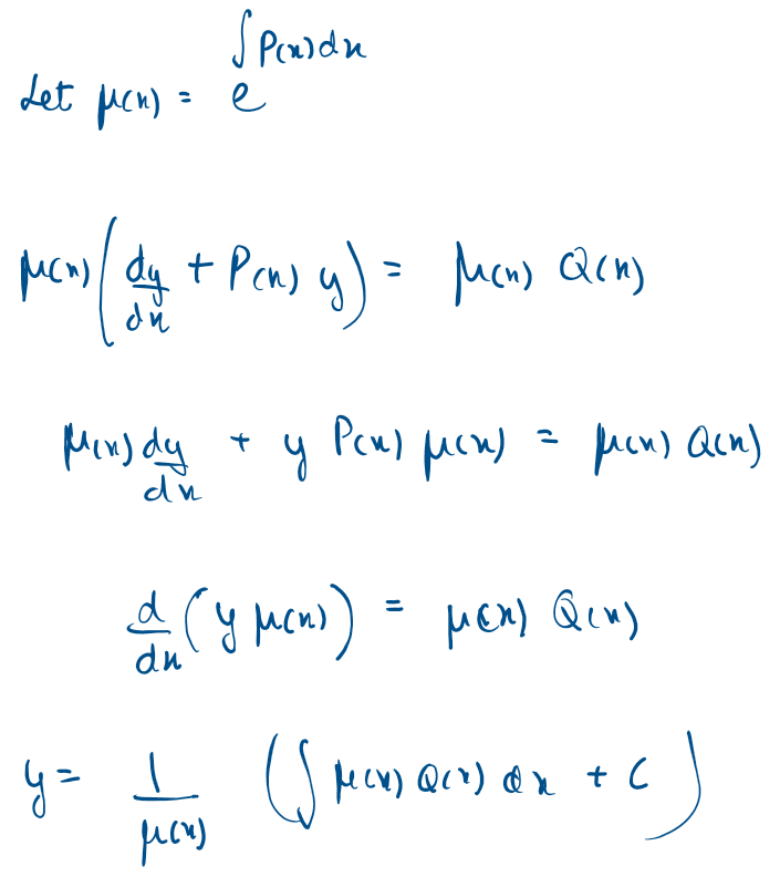
The intuition is to multiply both left and right hand side by a factor which would help resolve the derivative using a product rule, so separation of variables and integral is possible.

This is one of the examples of mathematical elegance showing how adding a seemingly complex functions can beautifully simplify the equation.

This “magic trick” however requires the differential equation to be strictly linear. If your dependent variable (y) is squared, or trapped inside a sine wave, the integrating factor shatters

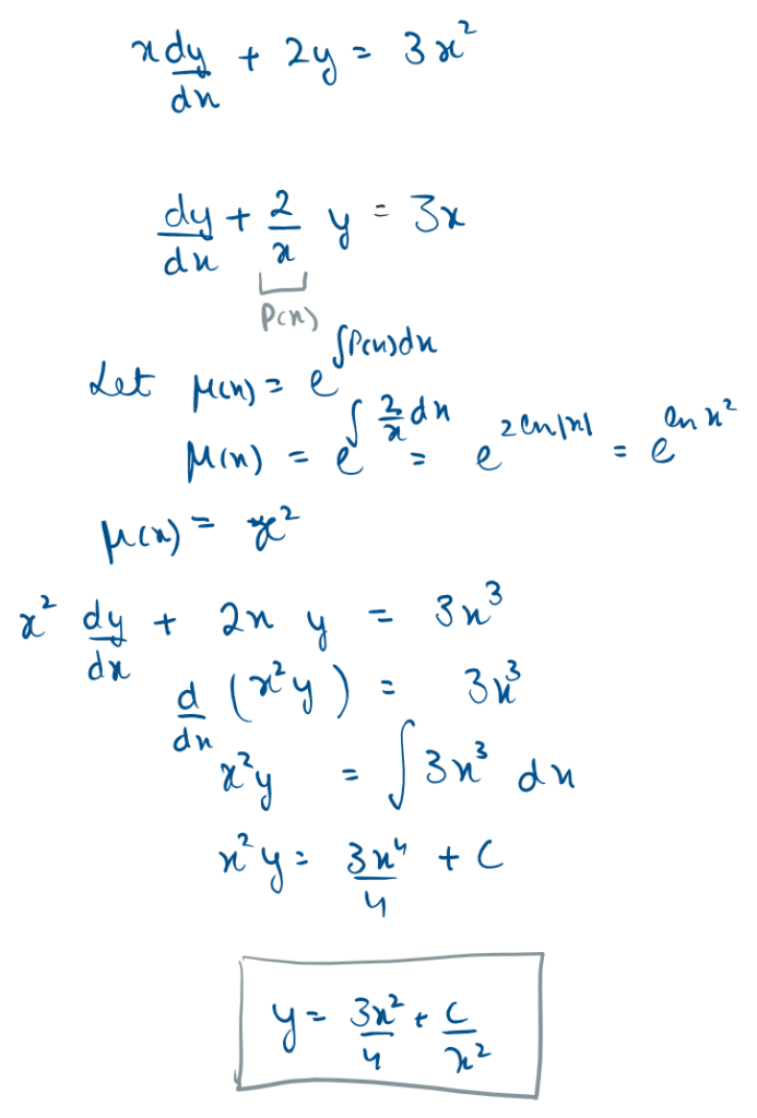
Lets walk through an example

Exact Equations

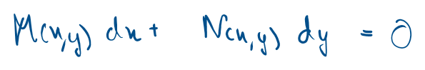
Can only be used if equation is exact

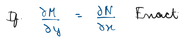
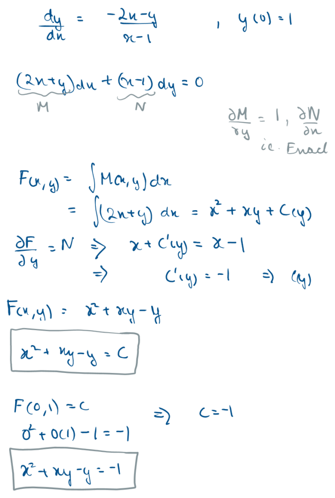
There is a general way to solve these kind of equations:

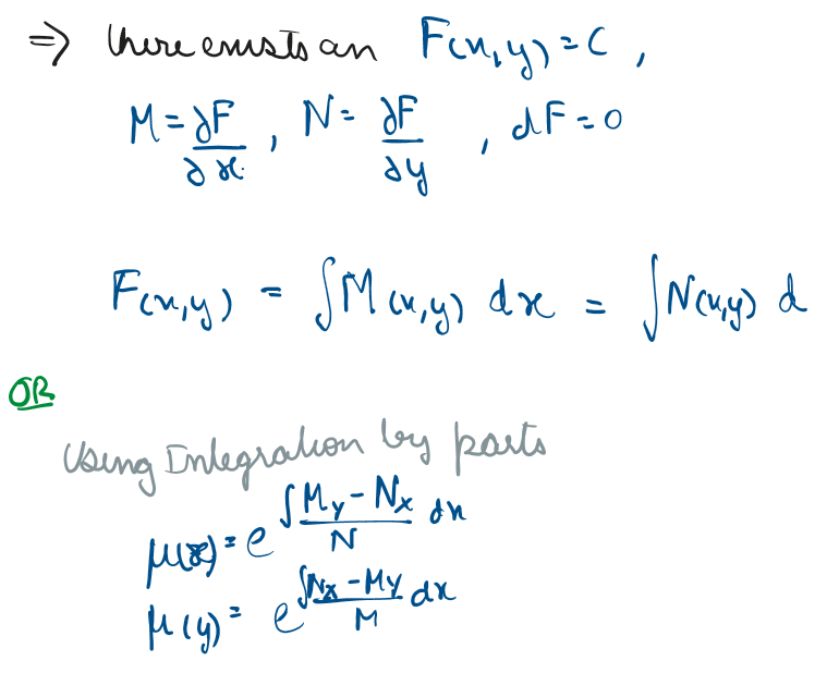
This method is deeply geometric. We use exact equations when our 1D differential equation is actually a shadow cast by a 2D topographical map, M and N are actually partial derivatives of the parent function F, hence, we are integrating the pieces we have to reconstruct the hidden parent function.

In physics, “exactness” often translates to conservative fields. If you are calculating the work done moving a satellite through Earth’s gravitational field, the energy required depends only on the start and end points, not the path taken. That gravitational field is an “exact” mathematical system

Bernoulli Substitution

Used for first order non linear equations

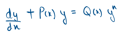
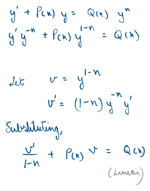
The intuition is to substitute using exponential of 1-n such that the equation can be converted into linear equation, this works for all values of n other than 0, 1

This is another example of mathematical elegance where we are basically disguising the system to look linear so we can solve it easily!

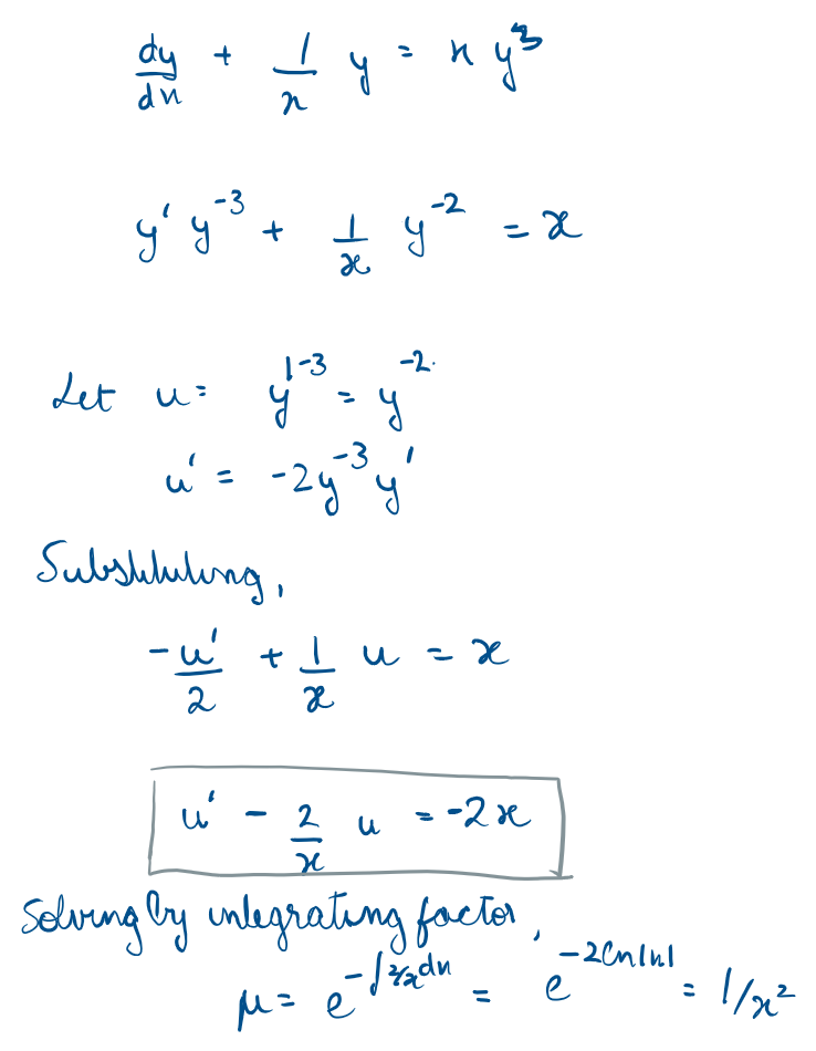
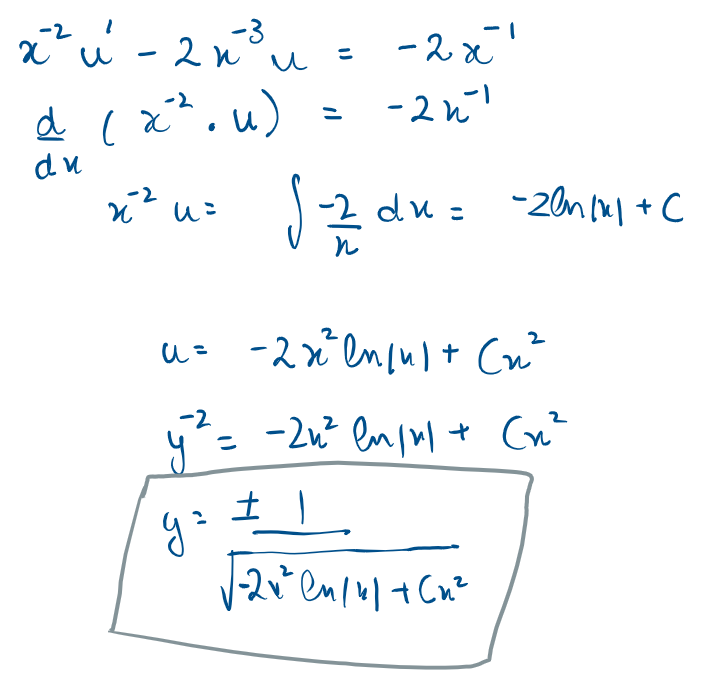
A general way of solving such equation would be:

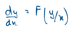
Homogenous Substitution

What homogenous here means that in this particular form, both numerator and denominator on the Right Hand Side have a degree of 1

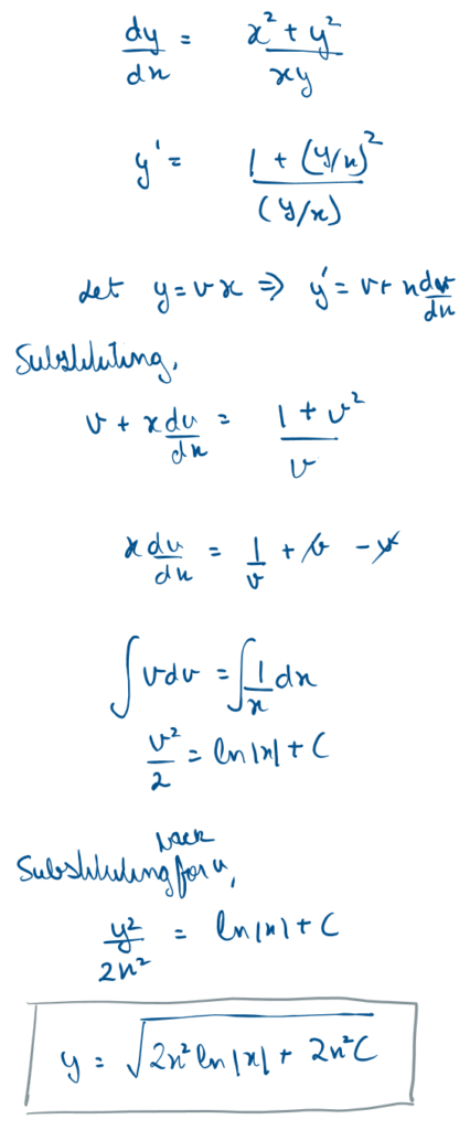
We actually work with these quite often assuming a linear relationship between x and y and converting the complex function such that the whole equation becomes separable

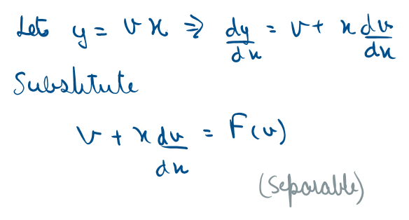
Which basically means that the whole system is scaling proportionally, Because the ratio between the variables is the only thing that matters, we stop trying to solve for y directly

This is highly relevant in fluid dynamics and thermodynamics, where the behavior of a system often depends on the ratio of properties (like density over pressure) rather than their absolute values

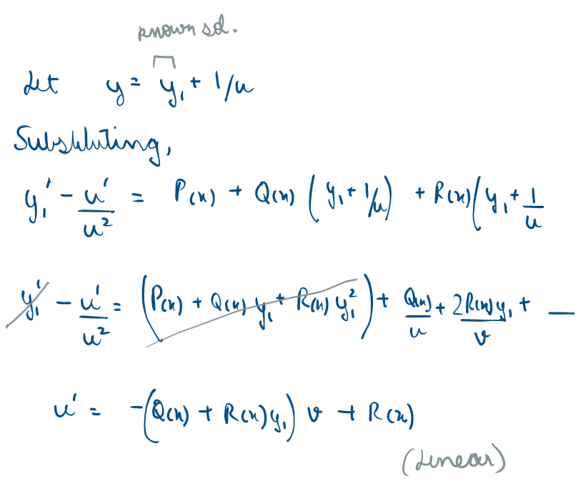
Riccati Substitution

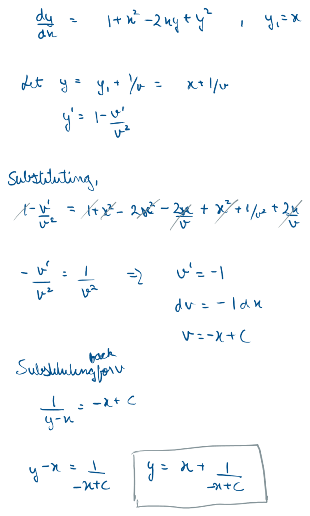
These are again used when our equations are first order and non linear (containing squared variable and given a known solution) a very specific use case and a notoriously difficult equation e.g.

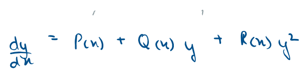
Like all substitution, the purpose is to simplify the equation to an easily solvable form, the specific substitution choice we make to this possible is as follows:

When a satellite is tumbling and needs to stabilize its attitude using reaction wheels, the onboard computer is actually continuously solving a matrix version of the Riccati equation to figure out the optimal torque to apply without overshooting, Riccati equations also frequently pop up in 1D gas dynamics and thermodynamics, specifically when modeling the flow of compressible gases through nozzles

References

3Blue1Brown – 8 Lecture Series on Geometric Intuition for Differential Equations