Wildfires are no longer just seasonal anomalies, they are increasingly frequent, destructive, and unpredictable global events. By the time a traditional satellite pass registers a thermal anomaly, a localized spark can already be a raging inferno. Today, the intersection of advanced Computer Vision, geospatial foundation models, and edge computing allows us to track wildfires from the moment they ignite to predicting their exact path of destruction.

You can look at this problem from different angles and different models that can help manage this problem from index/risk to active management with models from object detection, spread prediction to burn area estimation, I have outlined a few as follows:

Object Detection & Localization

Catching a fire in its infancy requires identifying microscopic smoke plumes across kilometers of dense forest. We will explore real-time bounding box localization designed for immediate alerting.

• Models: Lightweight edge models like YOLOv8n and YOLO11n, pitted against advanced transformer architectures like RS-DETR and RT-DETR-Smoke.
• The Data: Training on D-Fire (21,000+ early smoke/fire annotations), PyroNear (authentic watchtower noise and sun glint), and HPWREN continuous video streams.

Semantic Segmentation

Once a fire is detected, we need to understand its exact footprint. This installment covers dense pixel classification to map active flames, unburned fuels, smoke coverage, and post-fire burn scars.

• Models: State-of-the-art geospatial foundation models including IBM/NASA’s Prithvi-EO-2.0 (300M/600M parameters) and SatMAE, alongside Mask2Former and Swin-UNet.
• The Data: Multi-spectral analysis using Sen2Fire, Landsat-8 Burned Area benchmarks, and high-resolution drone thermal imagery from M4SFWD / FLAME.

Boundary Detection

Wildfire containment relies on knowing exactly where the fire line is right now. We will discuss extracting 1D active fire perimeters from complex topographical imagery.

• Models: Edge focused network architectures like BDCN, GSCNN, and SAM-Assisted Stochastic Extractors, PidiNet
• The Data: Aggregating thermal anomalies into concave hulls using MODIS/VIIRS Active Fire Vector Perimeters and the 30m resolution HLS Fire Perimeter Dataset.

Pixel Masking & Hotspot Classification

Not all fires produce visible smoke immediately. This post tackles pixel-wise and point-wise binary hotspot classification using thermal heuristics and infrared imagery.

• Models: Gradient boosting techniques (XGBoost, LightGBM) and 1D-CNNs applied to spectral indices like dNBR and MIRBI.
• The Data: Geostationary thermal IR imagery from GOES-16/18 ABI (FDC) with 5–15 minute refresh rates, and VIIRS 375m I-Band data.

Hybrid Spatiotemporal Spread Prediction

Where will the fire be in two hours? By fusing AI with environmental factors and physics, we can model the future.

• Models: Next-generation spread forecasting using UNet-FNO, Spatio-Temporal Mamba (ST-Mamba), and ConvLSTM
• The Data: Multi-modal benchmarks like WildFireSat and FireSpread / EarthNet, incorporating Sentinel-1 SAR (for cloud penetration), Sentinel-2 optical data, DEM topography, and ERA5 wind vectors.

In this post we focus on the first part – Object Detection

Flood work lived in Earth Observation space: Sentinel-1 SAR, elevation, HAND, weather vectors, pixel masks. Wildfire early warning from cameras is a different physics and a different label geometry. You care about where the plume is, not a per-pixel land-cover map so we start with a classic object detection: boxes for smoke and fire.

The goals for this iteration:

1. Explore the data and set up a repeatable train and evaluate on an extensive dataset like D-Fire
2. Compare two CNN nanos (YOLOv8n, YOLO11n) against two real time DETRs (RT-DETR-L, RF-DETR Nano)
3. Ask the deployment question : what actually fits an edge budget (size, latency, RAM) once the boxes look vaguely plausible

Data

We use D-Fire dataset which contains 21,527 RGB images, all standardized to 416×416 resolution, they all are annotated with bounding boxes following YOLO format (which are normalized between 0 and 1)

We have – “fire” (comprising 14,692 bounding boxes) and “smoke” (comprising 11,865 bounding boxes)

If you look at how those boxes are distributed across images:

• Smoke only: 5,867 images
• Fire only: 1,164 images
• Both Fire & Smoke: 4,658 images
• Background (Empty): 9,838 images

At first glance, having nearly 10,000 images with zero annotations might look like noise. In reality, this might be a critical feature for edge deployment. Watchtower cameras and drones constantly stream video of clouds, fog, horizon glare, and mountain ridges. If you train an object detector exclusively on images containing active flames, the model learns a strong prior that something must be in the frame, leading to constant false alarms. By including a massive proportion of negative samples, the model learns what not to trigger on, drastically curbing false positives in the field.

For test purposes however, we start small, we cap our training data at 512 images and val and test at 128 each

Here is what our split distribution looks like:

split	n_images	n_empty_bg	n_boxes	n_smoke	n_fire
train	512	238	636	270	366
val	128	52	168	82	86
test	128	52	171	74	97

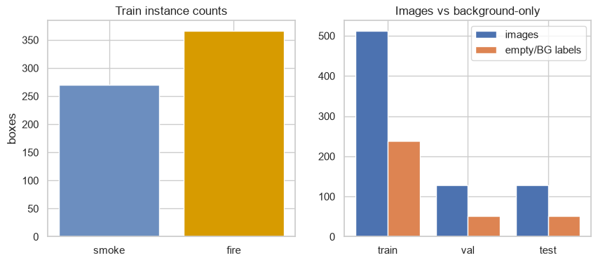
Left: As you see across all three splits, background-only images consistently account for 40% to 46% of the total frames (238/512 in train, 52/128 in val/test). This ensures our mini models are still trained and evaluated against hard negative samples (fog, clouds, horizon glare) rather than artificially over-saturated target frame and the bounding box count preserves the mild class imbalance seen in full D-Fire, maintaining roughly a ~1:1.35 ratio of smoke to fire instances (270 vs 366 in training)

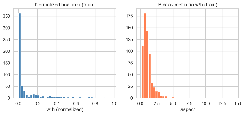
Right: remember the data is normalized between 0 and 1, the bounding box area distribution in the 512 image training sample remains overwhelmingly clustered near 0 (microscopic targets – size of fire in most frames < 1% of image), while aspect ratios (w/h) stay tightly bound between 0.8 and 1.5 (so its square rectangular bounding boxes – which is not very useful to know it seems but we can be assured at least its not a lot of 10s and 15s which would just be long thin boxes almost like lines confusing the model)

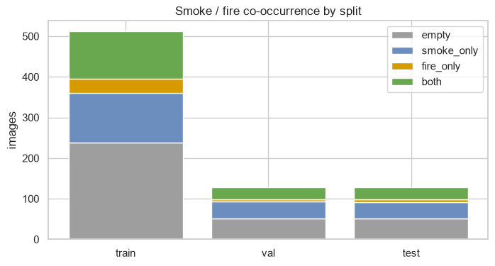
We also checked co occurence of fire and smoke particularly to look for “smoke-only” images (23.8% in train, 32.0% in val) – these will probably help more in early warning signals.

Then we look at object density per bin as there could be multiple instances / bounding boxes of fire in an image with an aggressive flare, thankfully our dataset is not too bad with most images contain only 1 to 5 boxes, this also means what we’re looking at is – isolated incidents or a few concentrated hotspots, rather than highly fragmented, scattered spot fires, even if we wanted to have that its not like we need to alter our data – the models we are using do use a parameter of max detections which we’ll discuss later.

Just for sanity we also checked IoU – and it was almost zero overlap. Even for smoke-fire pairs, only 0.3% have an IoU greater than 0.5, which means while smoke and fire coexist in the same image, the bounding boxes rarely overlap each other significantly. Smoke usually sits directly above the fire box, not over it

Here are some samples visualized:

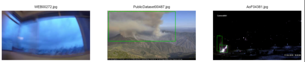
We look at the spatial distribution of these fire and smoke boxes across our samples and we find, for smoke, 10.4% of centroids in lower half (cy > 0.5); n=270 and for fire, 53.8% of centroids in lower half (cy > 0.5); n=366

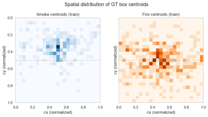
Which is kind of natural probably teaching the model spatial preference as well (look for smoke in the sky and fire at the ground), but keep in mind the data we train on has this bias, so if you a random vertical flip, or upside down drone there could be a horizon bias like this, we could fix it by sampling differently and by flipping / mosaicking images introducing noise and generalizing the model as per our requirements but we’ll skip all that on this iteration.

We also inspect box sizes and we find that – 29.5% of fire instances are “Small” (< 32×32 pixels), but only 1.5% of smoke instances are small, with a massive 77.8% classified as “Large”

This again is expected because while the smoke plumes look tiny compared to a vast mountain range, they actually occupy a large number of pixels because smoke diffuses and spreads. Fire, on the other hand, is genuinely microscopic in pixel term

class	bucket	count	pct	n_class
smoke	Small	4	1.481481	270
smoke	Medium	56	20.740741	270
smoke	Large	210	77.777778	270
fire	Small	108	29.508197	366
fire	Medium	172	46.994536	366
fire	Large	86	23.497268	366

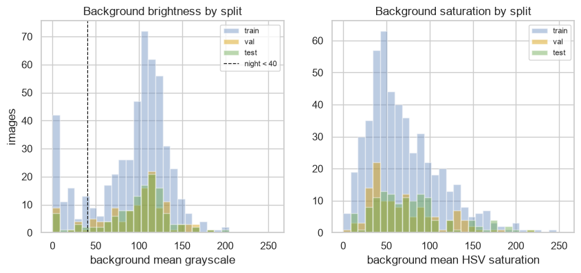
We also have another bias in our dataset, we checked brightness and saturation of our images and found out most of our images are actually daytime with only 10-16% night time ones, while this might not be a problem for the usecase where we’re operating in the daytime only but something to be kept in mind when evaluating the model and reporting its performance

Now, for data prep, YOLO and DETR require different formats, the D-Fire dataset is already optimized for YOLO, for the transformer, we convert the data to COCO format,

Feature	YOLO Format	COCO Format
File Structure	Decentralized: One .txt file per image	Centralized: A single .json file for the entire split
Bounding Box	Normalized: [class_id, x_center, y_center, width, height] (range 0.0 to 1.0)	Absolute pixels: [x_min, y_min, width, height]
Labels & Categories	Zero-indexed integers (0, 1, 2...) mapped via a data.yaml config	Explicit category dictionary mapped inside the JSON ("id": 1, "name": "fire")
Metadata	Minimal (only class ID and box coordinates)	Rich (image dimensions, licenses, segmentation polygons, keypoints, area)

Because of the nature of these models not just the input format is different but outputs are also different, YOLO for instance predicts a Results object and DETR returns a nested dictionary. so we standardize that as well having 3 NumPy arrays of boxes, labels and scores.

Models

To evaluate performance across different edge computing paradigms, we pit two CNN-based detectors (YOLO) against two Real-Time Vision Transformers (DETR).

To recap a classic object detection method say something like R-CNN used to scan the image for different regions of interest guessing where an object might be and then focus on each of those regions one by one and classify/label them, that’s the gist of it and as you can see it seems a highly cumbersome and slow process.

YOLO

YOLO (You Only Look Once) models have been the gold standard for real time edge vision for years. They rely on Convolutional Neural Networks (CNNs), which process images by passing filters over pixels to detect edges, textures, and eventually complex shapes.

CNNs are incredibly efficient because they focus on local pixel neighborhoods. This makes them blindingly fast and highly compressible.

Instead of scanning the image hundreds of times, YOLO takes the image and slaps a grid over it (like a giant chessboard). It looks at the entire image exactly one time. In that single glance, every single square on the chessboard simultaneously asks:

1. Is the center of a fire inside my square?
2. If yes, how wide and tall is the fire?
3. How confident am I?

We will try to dive into these architectures in detail in a separate post, for now a brief about the two versions we tried:

• YOLOv8n (Nano): Weighing in at just 3.01 million parameters, its native PyTorch checkpoint was a microscopic 5.96 MB.
  Also called an anchor free detection system, which means instead of predicting offsets from predefined anchor boxes like its predecessors (think of as fixed size stencils – which the model slides over whole image and finds the location and stencil that fits best), the model instead predicts the exact center of an object (looks for center pixel then finds the shape from center)
  Since each image is swept through grid by grid, this could lead to multiple overlapping boxes and there’s an additional cleanup step – Non Maximum Suppression (NMS) which suppresses other boxes.
  It also uses a focal loss function to give more weight to hard to detect objects (like microscopic fire plumes)
  In addition to all this, this generation of models also utilizes this technique called C2f – Cross Stage Partial Network with 2 convolutions and fusion which basically means splitting the image into two, sending one part for heavy analysis and the other to be fused back together in the end much like UNets skip connection (not really but lets say that for intuitive understanding right now) with the same purpose of not getting too distorted in the abstractions by too many convolutions
  
• YOLO11n (Nano): The latest iteration is even leaner at 2.59 million parameters and 5.21 MB in size.
  In this version C2f is replaced with C3k2 (Cross Stage Partial with kernel size 2) which is a more compressed way of doing it, this is to help further with processing speed.
  In addition, it introduces C2PSA (Cross Stage Partial Spatial Attention) instead of standard convolution layers treating features more or less equally, in this generation of model we have Channel Self Attention globally reweighting feature channels and deciding whats more important and Spatial Self Attention which looks at the actual pixel locations and re weights them based on their relevance to the object being detected.
  It also implements a Spatial Pyramid Pooling – Fast (SPPF) which as you guessed zooms and stretches image on various levels and pools them so models good with different visual scales.

Because CNNs focus locally, they struggle to capture the “global context” of an image. If a faint wisp of smoke looks like a cloud locally, a YOLO model might ignore it, leading to the high false-negative rates we saw in our EDA.

DETR

DETR (DEtection TRansformer) architectures abandon standard convolutions and instead use the Transformer architecture (specifically, self-attention mechanisms). Instead of just looking at local pixel grids, Transformers look at the entire image at once, learning how different patches of the image relate to one another.

By processing the global context of the image, the Transformer can understand that a gray blob is “smoke” because it is rising from a “forest” canopy, rather than just floating in the “sky”. Transformers however are mathematically expensive. The self attention calculations require significant memory.

DETR models are inherently NMS free, they predict a fixed set of bounding boxes directly, completely avoiding the messy overlapping-box cleanup step that YOLO requires.

• RT-DETR-L (Large): A heavy, highly accurate model boasting 32.81 million parameters and a native size of 63.1 MB.
  A Real-Time DETR starts with a traditional highly optimized CNN architecture like ResNet to create feature maps from the image, then its the feature map is handed to the transformer which separates “intra-scale” interactions (looking for details within the same zoom level) from “cross-scale” fusion (stitching big features and small features together)
  RT-DETR specifically instead of random object queries, looks at the CNN’s feature maps first, picks the highest-confidence spots, and uses those as the starting queries.
  
• RF-DETR Nano: A specialized architecture built to bring Transformer precision to real-time applications. It has a footprint of 115.20 MB in our tests.
  Instead of a CNN, it uses DINOv2, a Vision Transformer trained by Meta on millions of images so it natively understands depth, texture, and object boundaries at a foundational level.
  Then it also borrows the C2f Projector from the YOLO architecture helping create multi scale features
  To increase speed instead of 6 layer decoder, it uses 3 layer decoder with something thats called deformable cross attention, an optimized attention mechanism used in previous iterations of DETR models as well.
  To make up for the fact that the decoder is “shallow,” researchers use a trick during training where they feed the model multiple groups of queries simultaneously. The model learns incredibly fast during training, but drops the extra groups during inference, keeping it lightweight when deployed
  

Training and Evaluation

For this PoC we just ran 5 epochs, YOLO models (v8n, 11n) both trained under ~8minutes and RF DETR nano took about 1 hour to train and RTDETR took about 1.5 hours.

Comparing their performances against the same test set:

model	backend	precision	recall	mAP50	mAP50_95	pr_auc	mean_iou	train_time_s	n_test
yolov8n	ultralytics	0.479125	0.255991	0.200996	0.081364	0.791056	0.698794	467.422160	128
yolo11n	ultralytics	0.505848	0.201588	0.146710	0.066961	0.708125	0.736623	478.060133	128
rtdetr-l	ultralytics	0.357221	0.366397	0.313390	0.153597	0.445392	0.740918	5747.818019	128
rfdetr_nano	rfdetr	0.474138	0.643275	0.743036	NaN	0.743036	0.747139	3227.180146	128

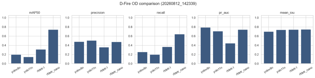
We notice a couple of things:

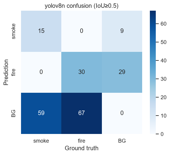
• YOLO models strongly favor precision (~0.5) over recall (~0.2) – when it predicts a fire, it is usually right but it completely misses roughly 80% of the targets
• RF DETR gave a respectable precision 0.474 while drastically boosting recall to 0.643
• RT DETR ‘s area under PR-AUC curve is the lowest of all 0.445

Mean Average Precision at an IoU threshold of 0.5 (mAP50) is the gold standard for object detection because it rewards models that both find the object and draw a tight box around it and RF DETR excels in that category

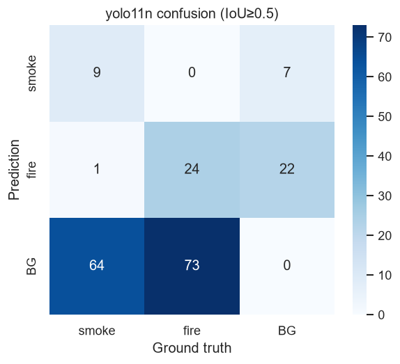
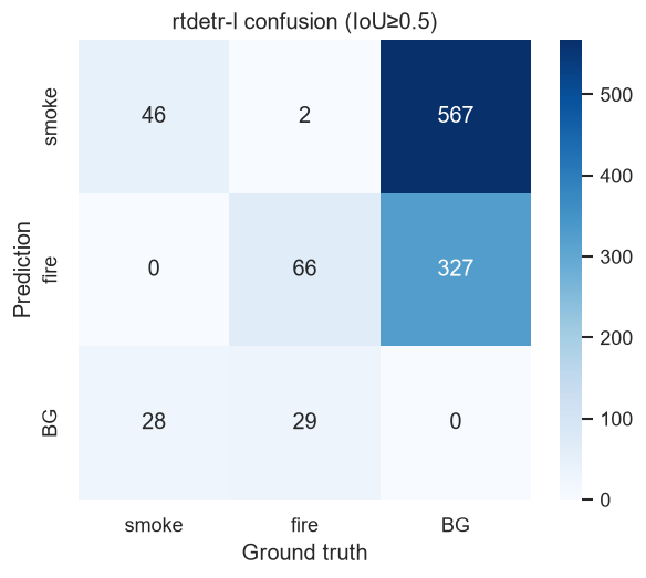
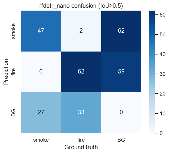
Edge Performance

We trained our models using PyTorch (even though YOLO was natively C or C++ – it was rewritten to PyTorch by Ultralytics which is the one we used) and RF DETR and RT DETR are both Transformer based models in PyTorch and by default we used Floating Point 32, to compress our model our first approach is quantization that is reducing that Float 32 precision of the saved weights of the trained model. Here we went from FP32 to INT8 reducing the size by ~4x, and subsequently freeing up RAM as well for inference.

Because we are squishing a wide range of continuous decimals into a tiny range of whole numbers (for example, INT8 only holds 256 possible values), the model has to introduce two new parameters per layer or block to help decode the integers, things like Scale Factor and Zero Integers

ONNX (Open Neural Network Exchange) is a standardized file format for Neural Networks (think like joblib or .pkl ), we can convert any model (PyTorch, TF, ScikitLearn) to ONNX, ofcourse there are other options like TFLite, ExecuTorch or some more specific ones like CoreML highly optimized for mobile hardware or even .cpp for LLMs if you were one of those first waves of running LLMs locally. You’d have probably heard of TensorRT – NVIDIA’s framework for its GPUs, they’re all in the same domain.

What they’re is a framework that takes in the trained model with all its weight, helps us quantize and delegate the math to the hardware in a highly efficient way – essentially helping us implement a ‘Lite’ version of the model we created, it brings with it lots of optimizations, memory management, orchestration efficiencies.

With Onnx RunTime (ORT) we have a hardware freedom (we’re not bound to NVIDIA or Intel as such) – and it does have a way to detect the hardware used and optimize for that, for instance if you were to use NVIDIA GPU it will use TensorRT in the back. It canrun in C/C++ environment and its a well established open source framework.

Now this is my first endeavor at edge frameworks and we don’t have hardware information / constraints yet so we start with the following basic evaluation strategy:

Metrics Considered

To determine if a model is viable for field deployment, we decided to look at the following hardware metrics:

• Disk / Flash Size (MB): Target is <= 50 MB. Field devices have highly restricted onboard storage. Smaller binaries also ensure faster, more reliable Over-The-Air (OTA) updates over weak cellular networks.
• Latency (ms) / FPS: Target is <= 100 ms (which translates to >= 10 FPS). Measured by running synthetic image tensors through the CPU over multiple timed iterations. This dictates real-time alerting capabilities; models must process frames fast enough to avoid dropping video feeds.
• Peak RSS RAM (MB): Target is <= 512 MB. Monitored using the psutil library. Edge microcontrollers share RAM with the OS and video pipelines. Exceeding this limit causes system crashes.
• Detection Quality (mAP50): High accuracy is required to ensure early smoke plumes and fires are caught

model	variant	size_mb	latency_ms	fps	peak_ram_mb	mAP50	params_m	compression_vs_fp32	edge_score
yolov8n	fp32_native	5.955	48.086	20.796	500.688	0.201	3.011	1.000	0.526
yolov8n	fp32_onnx	11.698	22.003	45.449	789.305	0.201	3.011	1.000	0.665
yolov8n	int8_onnx	3.200	162.171	6.166	913.051	0.201	3.011	3.655	1.156
yolo11n	fp32_native	5.214	47.827	20.909	697.836	0.147	2.590	1.000	0.649
yolo11n	fp32_onnx	10.114	19.144	52.237	823.789	0.147	2.590	1.000	0.668
yolo11n	int8_onnx	2.874	156.872	6.375	944.594	0.147	2.590	3.519	1.157
rtdetr-l	fp32_native	63.148	436.144	2.293	985.734	0.313	32.810	1.000	2.517
rtdetr-l	fp32_onnx	125.415	172.008	5.814	2034.777	0.313	32.810	1.000	2.734
rtdetr-l	int8_onnx	32.442	1673.848	0.597	2093.340	0.313	32.810	3.866	7.159
rfdetr_nano	fp32_native	115.200	166.291	6.014	1405.293	0.743	NaN	1.000	2.237
rfdetr_nano	fp32_onnx	111.375	72.045	13.880	1751.930	0.743	NaN	1.000	2.123
rfdetr_nano	int8_onnx	35.290	75.604	13.227	1721.977	0.743	NaN	3.156	1.608

The yolov8n in its raw fp32_native PyTorch format was the only model in its raw form to successfully pass all edge budgets we set, using 500.69 MB of RAM with an inference latency of ~48 ms.

ONNX boosted speed but devoured RAM, exporting to fp32_onnx dramatically accelerated the YOLO models. For instance, yolo11n latency dropped from ~47.8 ms to ~19.1 ms (achieving ~52 FPS). However, the ONNX Runtime caching pushed yolo11n‘s RAM usage to 823.79 MB, causing it to fail the 512 MB memory budget

The rfdetr_nano model dominated the accuracy metric with an mAP50 of 0.743. Yet, Transformers are mathematically heavy, its ONNX variant required over 1751 MB of RAM and ~72 ms of latency, meaning it requires a much larger edge gateway to run successfully, the int8 quantizationt maintains the superior 0.743 mAP50 and processes at 13.22 FPS, drastically shrinks its storage footprint from 111.3 MB down to just 35.29 MB (a 3.15x compression) but the RAM consumption is still fairly high. This is ideal if your edge device has plenty of RAM but very limited flash storage for OTA updates.

Conclusion

Achieving an mAP50 of 0.743 and a recall of 0.643, its DINOv2 Vision Transformer backbone excels at using global context to identify faint smoke plumes that local CNNs miss. Quantizing it to INT8 ONNX slashes flash storage from 111.3 MB down to 35.3 MB (~3.15x compression) while maintaining 13+ FPS. However, its ~1.7 GB RAM footprint requires an edge gateway rather than a low-power microcontroller.

Achieving ~19 ms latency (52 FPS) under FP32 ONNX with a microscopic 5.2 MB binary, YOLO11n is the only architecture that comfortably meets tight memory and power budgets out of the box

Due to the strict 5-epoch limit of our sandbox environment, the YOLO models were stopped prematurely. Looking at the training history plots, the validation mAP curves for both YOLOv8n and YOLO11n show massive, uninterrupted upward momentum. The models were shut off right as they were rapidly learning to identify microscopic smoke plumes.

The Next Step: Before we commit to heavy, RAM-hungry edge hardware to support a Transformer, our next milestone is a 150 epoch training run on a larger data sample as well. A fully converged YOLO11n with its microscopic 5.2 MB footprint and 50+ FPS throughput might just be the holy grail that satisfies both our accuracy requirements and our strict edge power budgets. But we’ll give RF-DETR and RT-DETR models another chance with the same data and more epochs and look into other quantization strategies/adapters for transformer models if the performance still drastically different.

References

• D-Fire Dataset — D-Fire: A Large-Scale Image Dataset for Fire and Smoke Detection
• R-CNN — Rich Feature Hierarchies for Accurate Object Detection and Semantic Segmentation
• Focal Loss — Focal Loss for Dense Object Detection
• Self-Attention Mechanism — Attention Is All You Need
• RT-DETR — DETRs Beat YOLOs on Real-Time Object Detection
• RF-DETR — RF-DETR: Neural Architecture Search for Real-Time Detection Transformers
• Ultralytics YOLO (v8 / 11) — Ultralytics Computer Vision Models and Documentation
• PyroNear — PyroNear: Open-Source Early Wildfire Detection Platform
• HPWREN — High Performance Wireless Research and Education Network Wildfire Cameras
• Roboflow RF100-VL — RF100-VL: Evaluation Benchmark for Vision-Language and Detection Models